Contribution of surface wave-induced vertical mixing to heat content in global upper ocean*
CHEN Siyu QIAO Fangli HUANG Chuanjiang SONG Zhenya
1 Ocean University of China, Qingdao 266100, China
2 First Institute of Oceanography, Ministry of Natural Resources, Qingdao 266061, China
3 Laboratory for Regional Oceanography and Numerical Modeling, Qingdao National Laboratory for Marine Science and Technology, Qingdao 266237, China
4 Key Laboratory of Marine Sciences and Numerical Modeling, Ministry of Natural Resources, Qingdao 266061, China
Abstract Compared with observations, the simulated upper ocean heat content (OHC) determined from climate models shows an underestimation bias. The simulation bias of the average annual water temperature in the upper 300 m is 0.2°C lower than the observational results. The results from our two numerical experiments, using a CMIP5 model, show that the non-breaking surface wave-induced vertical mixing can reduce this bias. The enhanced vertical mixing increases the OHC in the global upper ocean (65°S-65°N).Using non-breaking surface wave-induced vertical mixing reduced the disparity by 30% to 0.14°C. The heat content increase is not directly induced by air-sea heat f luxes during the simulation period, but is the legacy of temperature increases in the f irst 150 years. During this period, additional vertical mixing was initially included in the climate model. The non-breaking surface wave-induced vertical mixing improves the OHC by increasing the air-sea heat f luxes in the f irst 150 years. This increase in air-sea heat f luxes warms the upper ocean by 0.05-0.06°C. The results show that the incorporation of vertical mixing induced by nonbreaking surface waves in our experiments can improve the simulation of OHC in the global upper ocean.
Keyword: surface wave-induced; vertical mixing; upper ocean heat content; air-sea heat f luxes; climate model
1 INTRODUCTION
The ocean plays a considerable part in the global energy budget because it is the primary heat reservoir for climate change (global warming), as it stores more than 90% of the excess heat (Palmer and McNeall,2014; Von Schuckmann et al., 2016). The variations of ocean heat content (OHC) are essential elements of the global and regional climate variability (Jin, 1997;Meehl et al., 2011; Roberts et al., 2015) and the transient response to climate change (Kuhlbrodt and Gregory, 2012; Geoff roy et al., 2013). The OHC variation has become an important indicator of climate change and its variability (Abraham et al.,2013).
Changes in the OHC also represents the global energy imbalance caused by anthropogenic climate change, and thus projections of future changes in this quantity need to be as accurate as possible for the projection of future global temperature changes and sea level rises. However, numerical models, including ocean general circulation models, coupled climate models, and earth system models, have def iciencies in simulating the OHC (Gregory et al., 2004; Achutarao et al., 2007). Previous studies have suggested that including volcanic forcing (Church et al., 2005;Gleckler et al., 2006) and other variable climate forcings can improve the simulation of the climate models (Delworth et al., 2005). Numerous studies have shown an increase in the global OHC over the past few decades (Abraham et al., 2013).
Involving the important physical processes of the real ocean is a part of the unremitting development of numerical models. The more attention of including the oceanic surface waves in the climate system has recently received (Huang et al., 2012, 2014; Qiao et al., 2013; Fan and Griffi es, 2014). Recent research found that wave-induced mixing can change the OHC in both ocean models (Stoney et al., 2018) and climate coupled models (Chen et al., 2018). Nevertheless, the vertical mixing does not create, but redistributes,heat.
In the present study, we focus on understanding the mechanisms underlying the changes in OHC in the upper ocean caused by surface wave-induced vertical mixing (which we henceforth refer to simply as Bv,for convenience). Domingues et al. (2008) compared the linear trend in ocean heat content in the upper 700 m and 300 m, and found that 91% of it stored in the upper 300 m. Adopting the same def inition as used in previous studies (Domingues et al., 2008;Balmaseda et al., 2013; Williams et al., 2015), we consider 0-300 m as the object of study in this research. Using two identical numerical experiments,one with and one without Bv, we reveal how incorporating the eff ects of Bv improves the simulation of the OHC in the global upper ocean. The paper is organized as follows. The numerical models and data are described in Section 2. The results are presented in Sections 3, and the main conclusions are summarized in Section 4.
2 MODEL, DATA AND METHOD
2.1 The setup of numerical experiments
The FIO-ESM (First Institute of Oceanography Earth System Model), developed by Qiao et al. (2013),was used to carry out the numerical experiments in this paper. FIO-ESM comprises coupled physical climate and carbon cycle models. The details of the FIO-ESM can be found in Qiao et al. (2013).
Two experiments, one with Bv and the other without, were performed to identify the contribution of Bv to the heat content in the global upper ocean.FIO-ESM was used for the two numerical experiments.Bv is expressed analytically as:

whereαis a constant set to 1 following Qiao et al.(2013),E(k→) is the wave number spectrum,ωis the wave angular frequency,k→ is the wave number, andzis the vertical coordinate axis (upward positive) withz=0 at the mean surface.
The experiment incorporating Bv adopts the numerical experiment design and forcing data recommended by the CMIP5 (Coupled Model Intercomparison Project Phase 5). A historical run was conducted for the 1850-2005 period to match the run period of the physical climate model. The other run was identical, except for Bv being not included.We chose the 20-year averaged model results (1986-2005) for the comparison of OHC simulations with Bv, and without Bv.
2.2 Observation data
The EN4 (Good et al., 2013) 1985-2006 objective analysis temperature data set was used to evaluate the upper ocean thermal content. In addition, we compared this climatological data with the World Ocean Atlas (2009) data (Locarnini et al., 2010); the results of the two data sets were almost the same.
2.3 Method
We calculated the upper OHC, integrated between the surface and the depth of 300 m, using:

whereTis the potential temperature,xis the zonal dimension,yis the meridional dimension,zis height,tis time, andcpandρ0are the heat capacity and density of sea water, respectively. In spherical coordinates:

whereRis the radius of the Earth,φis latitude, andθis longitude. The OHC can be intuitively characterized as the average temperature.
The geographical distribution of OHC can be characterized by the vertically-integrated temperature(VIT, units: m°C). We calculated VIT using:

whereTais the climatological monthly average temperature for the period 1986-2005.
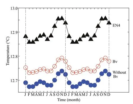
Fig.1 Climatological monthly average temperature of the upper ocean (0-300 m) between 65°S and 65°N during the simulation period (1986-2005)
3 RESULT
3.1 Eff ects of Bv on the simulation of OHC
Here we investigated the OHC using the average temperature in the 0-300 m layer. Figure 1 shows the climatological monthly average temperature of the upper ocean over the simulation period (1986-2005).The mean of the EN4 data set was 12.90°C and the mean of the case without Bv was 12.70°C. The mean temperature rose to 12.76°C when Bv was included.The global average temperature of the upper ocean increased by almost 0.06°C when incorporating Bv,and was closer to the observational data. Thus, the simulation bias (0.2) was improved by 30% (to 0.14)when Bv was included.
Figure 2 shows the VIT in the upper ocean (0-300 m), and illustrates the geographical distribution of the OHC. The simulation bias compared to the EN4 data is highly variable in space. Although it appears that, overall, there is a negative bias for the case without Bv (Fig.2b) and the case with Bv(Fig.2c). However, there are slight positive biases in regions along the coast of North America in the Pacif ic Ocean, the northern Indian Ocean, and in some places in the Southern Ocean. Figure 2d shows the diff erence in VIT for the cases with and without Bv. The VIT signif icantly increased because of the inclusion of Bv in most areas, but not in the tropical western Pacif ic Ocean. However, in the equatorial Indian Ocean and the western Pacif ic Ocean, the reduced VIT increased model errors.
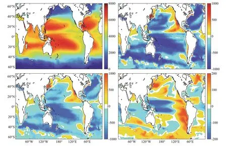
Fig.2 Vertically-integrated temperature and simulation biases (m°C)
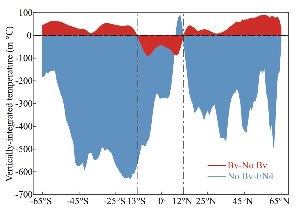
Fig.3 Diff erences in the zonally-averaged, verticallyintegrated temperature (0-300 m)
Figure 3 shows the result of the zonally-averaged vertically-integrated temperature. From the f igure, we can see that the simulated OHC without BV is less than that in EN4. Because Bv typically increases the local OHC by changing the vertical mixing and stratif ication, improvements in the simulation tend to occur in those regions that have pre-existing negative biases. The latitude band between 13°S to 12°N is an exception to this rule. However, the reduced OHC in the latitude band between 7°N and 12°N seems to reduce the model errors of the case without Bv.
3.2 Mechanism by which Bv aff ects OHC simulation
As is generally known, vertical mixing cannot generate heat but redistributes it vertically. In the coupled climate model, the air-sea heat f lux acts as part of the source of heat. We investigated the zonallyaveraged net surface heat f lux during the simulation period (Fig.4). We found that the zonally-averaged net surface heat f lux was very close for the two cases.The model is equilibrated, and the mean value of the diff erence of the annual mean net surface heat f lux is almost zero (0.02 W/m2). Therefore, it is reasonable that the values of the zonally-averaged net surface heat f lux for the two cases are close. However, in terms of heat content, the diff erence should be ref lected in the net surface heat f lux. Therefore, we consider that the change should be ref lected in the initial period when Bv is included.
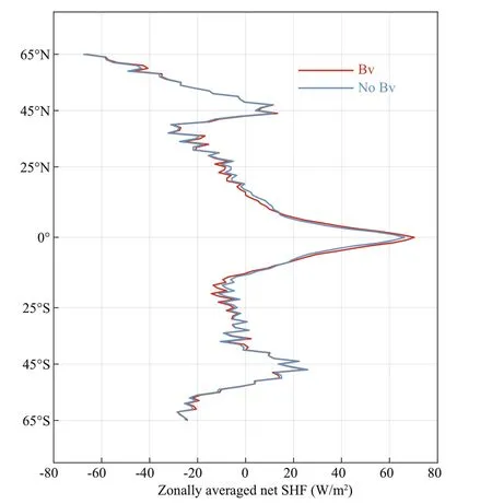
Fig.4 Zonally-averaged net surface heat f lux during the simulation period (1986-2005)
The numerical experiment design and forcing data recommended by the CMIP5 were adopted in the experiment that includes Bv. A historical run for the period 1850-2005 was conducted to match the period of the climate model. The other run was identical,except that Bv was closed. A control run for the preindustrial period (before 1850 AD) integrates the coupled physical climate model for 1200 years with the constant forcing f ields of greenhouse gases,aerosol, and solar irradiance from 1850. Model year 701 was chosen as the initial state for the historical integration of 1850-2005 (Qiao et al., 2013). We chose the f irst 200 years of the control run, when Bv is f irst included.
Figure 5 shows the time evolution of the diff erence in the global average net surface heat f lux between the cases with and without Bv in the f irst 200 years. We found that the global average net surface heat f lux increased when Bv was included in the f irst 150 years.For the following 50 years, the diff erence in net surface heat f lux f luctuates around zero.
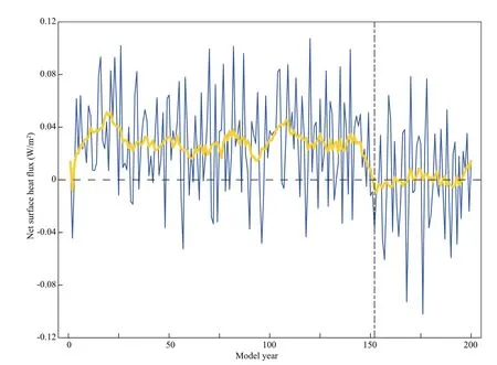
Fig.5 Time evolution of the diff erence in the global average net surface heat f lux
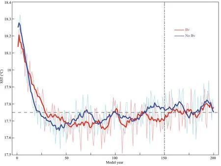
Fig.6 Evolution of the annual-mean global averaged SST in the pre-industrial period according to the climate model
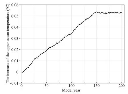
Fig.7 Increases in upper ocean temperature caused by changes in the surface heat f lux
In coupled climate models, the surface heat f lux has a negative feedback with the sea surface temperature (SST). Figure 6 shows the global annual mean SST over 0-200 years. We found that, when Bv was included, the SST was higher than when Bv was closed in the f irst 150 years, especially in the 50-150-year period. This occurs because the increased mixing can transport more heat from the surface to the subsurface, thereby cooling the SST. The lower SST leads to an increased surface heat f lux into the ocean,and the increased vertical mixing can transport the heat eff ectively, and warm the upper ocean. If the surface heat f lux increases continuously, then the OHC will increase linearly. This is not reasonable.The climate model is a coupled system, and after a 150-year adjustment, it adjusts to an equilibrium state. The SST reaches a dynamic equilibrium state,with small f luctuations around an average value of 17.73°C, which is close to the observed value of 17.88°C in 1850 obtained from the Hadley Centre Sea Ice and Sea Surface Temperature dataset (HadISST)(Rayner et al., 2006).
The increase in the surface heat f lux induced increases in the upper ocean temperature as shown in Fig.7. The accumulated net heat f lux heats the upper 300 m of ocean by 0.05-0.06°C; this accords with the results shown in Fig.1.
4 SUMMARY AND CONCLUSION
In this study, we evaluated the contribution of Bv to the heat content in the global upper ocean. The mean temperature of the upper ocean was improved from 12.7°C to 12.76°C, and was closer to the EN4 observational results (12.9°C). By including Bv in the model, the diff erence in the upper ocean temperature was reduced from 0.2°C to 0.14°C. Thus, the inclusion of Bv reduced the diff erence for about 30%.
We analyzed the net surface heat f lux for the simulation cases that included and without Bv during the experiment period, and the diff erence in the results is quite small. The increase in OHC by inclusion of Bv, however, was not caused by changing the surface heat f lux during the experiment period. We found that the surface heat f lux was higher for the f irst 150 years after Bv was initially included in the climate model.The surface heat f lux and SST then reached a dynamic equilibrium state. We integrated the increase of the surface heat f lux induced by the change of the upper ocean temperature. We found that the increase in the upper ocean temperature was 0.05-0.06°C, which is consistent with the increase from 1986-2005. Thus,the increase in the temperature in the system is the legacy of temperature increases in the f irst 150 years when Bv was initially included in the climate model.
We observed that the simulation of OHC was worse in the tropical regions (13°S-10°N) when Bv was included. In addition, the simulation of OHC when Bv was included was lower than that when Bv was closed. This may be because other physical processes dominate in the simulation of the tropical OHC in some regions. Because of the importance of OHC,further investigations are required to study the reasons for this discrepancy.
5 DATA AVAILABILITY STATEMENT
Data supporting this article are available by any users from http://data.f io.org.cn/qiaof l/CSY-JGR-2018.
 Journal of Oceanology and Limnology2020年2期
- Journal of Oceanology and Limnology的其它文章
- Upper ocean response to typhoon Kujira (2015) in the South China Sea by multiple means of observation*
- Inf luence of simulating deep-sea environmental factors on cathodic performance of seawater battery*
- Adsorption characteristics of chitooligosaccharides onto activated charcoal in aqueous solutions*
- Eff ects of hypoxia on survival, behavior, and metabolism of Zhikong scallop Chlamys farreri Jones et Preston 1904*
- Distinct inf luence of trimethylamine N-oxide and high hydrostatic pressure on community structure and culturable deep-sea bacteria*
- Microbial communities present on mooring chain steels with diff erent copper contents and corrosion rates*
