Changes in the phytoplankton community structure of the Backshore Wetland of Expo Garden, Shanghai from 2009 to 2010

Xuemei Miao, Shaokun Wang, Mengqun Liu, Jie Ma, Jian Hu, Tianli Li,Lijing Chen,*

a National Demonstration Center for Experimental Fisheries Science Education, Shanghai Ocean University, Shanghai, 201306, China

b Key Laboratory of Freshwater Aquatic Genetic Resources, Ministry of Agriculture, Shanghai Ocean University, Shanghai, 201306, China

c Shanghai Collaborative Innovation for Aquatic Animal Genetics and Breeding, Shanghai Ocean University, Shanghai, 201306, China

Keywords:Backshore wetland Phytoplankton Community structure Environmental factor

ABSTRACT Phytoplankton community structure,abundance,and species'spatial and temporal distributions were examined for the Backshore Wetland of Expo Garden in Shanghai from September 2009 to August 2010. A total of 371 phytoplankton species were identified from 109 genera 8 phyla. There were 18 dominant species in total, and Phormidium tenue was dominant during four seasons. The mean annual abundance and biomass were 711.11×104 cells/L and 5.70 mg/L, respectively. The seasonal changing trend of existing stocks was bimodal,with main peaks of density and biomass occurring in the winter and a secondary peaks occurring in the summer.The Shannon-Wiener diversity index(H′),the Margalef species richness index(D),and Pielou's species evenness index(J)showed a clear seasonal trend.All of the indices showed a changing pattern,with the highest recorded values from the summer to autumn and the lowest recorded values from the winter to spring. The canonical correspondence analysis (CCA) showed that environmental factors, including water temperature, nitrate nitrogen, and pH were the main influencing factors to the change of phytoplankton community structure in the Backshore Wetland of Expo Garden in Shanghai.

1. Introduction

As the primary producers of aquatic ecosystems, phytoplankton plays a vital role in the energy flow, material circulation, and information transmission in freshwater ecosystems(Li,Li,&Wang,2007;Zhang&Song,2006).Compared to other aquatic plants,phytoplankton biomass and community structure can better reflect water quality status and trends, especially changes in nutrient levels, because they have short growth cycles and are sensitive to rapid changes in the water environment. It is an important indicator for evaluating the quality of the water environment (Huang, 2001; Lin, Hu, & Duan, 2003; Rott &Cantonati,2006;Sidik,Nabim,&Hoque,2008).Conversely,changes in environmental conditions can also directly or indirectly affect phytoplankton community structure.

Currently, phytoplankton species account for 25% of all aquatic species used to indicate water quality. Phytoplankton plays an important part in biological monitoring and the evaluation of water pollution and nutrient levels, which has been effectively and widely used domestically and abroad(Marchetto,Padedda,&Marinani,2009;Song,Liu, & Pan, 2007; Tan, Kong, & Zeng, 2009). Research on how to use phytoplankton to control water pollution has also been reported(Comin, Menendez, & Lucena, 1990; Lu, Yao, & Zhou, 1992). The differences of phytoplankton community structure determine the differences of ecosystem foundations. Understanding phytoplankton community structure is the basis of research on succession, community function,classification,distribution,and the environment(Song,2001).Therefore, research on the response of phytoplankton to the ecological restoration of the Backshore Wetland can provide the basic data and theoretical support for understanding phytoplankton community structure.

2. Materials and methods

2.1. Sampling sites and time

The Backshore Wetland water system was formed by integrating raw water introduced into the Huangpu River and natural precipitation through a matrix filtration with adsorption, precipitation,nitrogen and phosphorus removal,heavy metal adsorption,and wetland purification.The samples were collected monthly at ten designated sampling stations(Fig. 1). Sample collection started in September 2009 and continued until mid-August 2010.

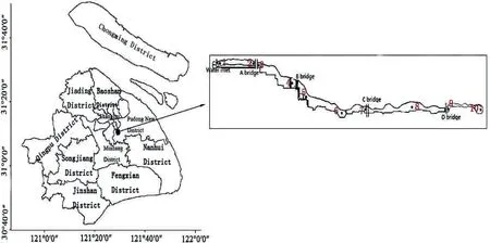
Fig. 1. Sampling sites of phytoplankton in the Backhore Wetland of Expo Garden in Shanghai.

2.2. Methods

Qualitative samples were collected with 25# plankton nets (mesh diameter 64 μm) that were slowly dragged on the surface of the water along an eight-shaped path(∞).Since the water depth of the Backshore Wetland is about 2 m,10 L of surface water(0.5 m depth)was collected for quantitative samples with a 5 L Plexiglass water sampler. One liter of water was fixed on-site with Lugol's solution and taken to the laboratory for further analysis. After precipitating in the laboratory for 48 h,the solution was concentrated to 50 mL and stored in 4%formalin for microscopic examination (Hu & Wei, 2006; Huang, Hu, & Wu,1985).

A 0.1 mL Lugol's subsample was taken for taxonomic identification and enumeration (cells/L) with an Olympus CX21, 400X microscope.Counts were completed two or more times in sequence (error range ≤15%). We calculated the average of counts each time, expressed as the number of phytoplankton cells per liter of water. The identification of phytoplankton species was completed using descriptions of species found in the literature (Danilov &Ekelund, 1999;Ditty&Shaw,1992).While identifying species,the geometric length of each species was measured and the corresponding geometric volume formula was used to determine the volume of each phytoplankton. The biomass of the species was then determined according to the fresh weight of phytoplankton at 109μm3=1 mg (Zhang & Huang, 1991). For species that were commonly found in the samples, 30 individuals were measured and the average of their geometric lengths was used. For rare species, biomass was calculated by averaging the number of occurrences for a species.

The water temperature[WT],pH,dissolved oxygen[DO],and other water quality factors were measured by YSI 6600EDS, the depth [D]was measured with a sounder,and the Secchi depth[SD]was measured with Secchi disc. At the same time, 1 L of water was collected for the analysis of additional parameters, including permanganate index(CODMn), five-day biochemical oxygen demand (BOD5), total nitrogen(TN), nitrate nitrogen (NO3-N), nitrite nitrogen (NO2-N), ammonia nitrogen (NH4-N), total phosphorus (TP), and phosphate phosphorus(PO4-P). These parameters were determined in accordance with standard methods(Wei,2002,pp.88-284).We used an acetone method(Zhang & Huang, 1991) to measure the concentration of chlorophyll-a(Chl. a).

2.3. Biodiversity index calculations

(1) Shannon-Wiener diversity index (H′): a comprehensive index of species richness,and a measure of the uniformity of the distribution of individuals, which reflects the degree of complexity and the stability of community structure. This index is described by the following formula: H′=-∑(ni/N)×ln (ni/N);

(2) Margalef richness index(D):reflects the richness of species number and individuals. D = (S - 1)/ln N;

(3) Pielou's evenness index(J):reflects the evenness of the individual's distribution among species. J=H′/ln S;

(4) Degree of dominance (Y) (Xie, Fu, & Liu, 2004): Y = (ni/N)×fi.

Where ni is the density of the ith species at one site, N is the total density,S is the total number of species,and fi is the appearance rate of the ith,Y is the abundance of species.A species is considered dominant if Y is greater than 0.02.

2.4. Data processing and analysis

SPSS 18.0 and CANOCO4.5 used for statistical analysis.Comparisons between bio-density and biomass among the sites were performed by using one-way ANOVA. Pearson correlation analysis and Canonical Correspondence Analysis (CCA) were used to analyze the relationships of species number, existing quantity, and the environmental factors. The phytoplankton density index was used to represent the relationship between the phytoplankton species and the environment. Phytoplankton density and the environmental data were subject to log10(x + 1) conversion processing. The CANOCO4.5 package was used to analyze and make bi-order maps of the species and the environmental factors.

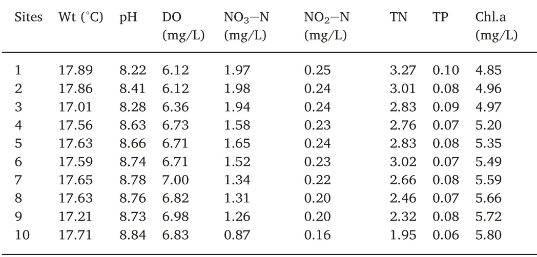
Table 1 Environmental parameters of the Backshore Wetland of the Expo, Shanghai,between September 2009 and August 2010.

3. Results

3.1. The physical and chemical factors

The main environmental factors of the Backshore Wetland of Expo Garden in Shanghai from September 2009 to August 2010 are shown in Table 1.

3.2. Phytoplankton species composition

A total of 371 species belonging to 8 phyla and 109 genera of phytoplankton were identified in the Backshore Wetland of the Shanghai Expo Garden (including variants). Among them, the number of Chlorophyta species was the highest(159 species)and accounted for 42.86% of the total number of species. Bacillariophyta followed with 105 species, accounted for 28.30%; Euglenophyta (56 species) accounted for 15.09%; Cyanophyta (38 species) accounted for 10.24%;and the number of Chrysophyta species was the smallest with only 1 species, which accounted for 0.27%. The Chlorophyta, Bacillariophyta,and Euglenophyta of the species found accounts for 86.49% of all phytoplankton species (Fig. 2).

The number of species varied seasonally,and was highest during the summer, followed by spring, autumn, and winter (Table 2). Chlorophyta and Bacillariophyta species were dominant during all seasons,while there was little variation in the number of Cyanophyta species among seasons.The number of Euglenophyta species only exceeded the number of cyanobacteria during the summer.

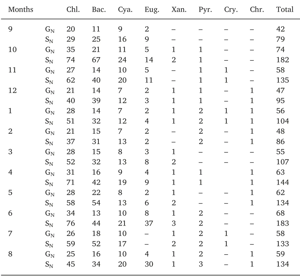
Table 2 Numbers of genera (GN) and species (SN) of phytoplankton in the Backshore Wetland of Expo Garden Shanghai.

3.3. Seasonal changes of dominant species

During the survey period, 18 dominant species emerged in the Backshore Wetland, belonging to Cyanophyta (6 species),Bacillariophyta (5 species),and Chlorophyta (7 species).The dominant species of phytoplankton showed similar seasonal succession patterns,while there were some differences in the number of dominant species during different seasons (Table 3). Among them,Phormidium tenue was the most dominant in autumn, spring, and summer (Y=0.38, 0.31,0.19, respectfully). In the winter, Gloeocapsa punctata was the most dominant (Y=0.38).

Phormidium tenue was a dominant species during all four seasons(Table 3).The dominance of Phormidium tenue was greatest in autumn,followed by spring, summer, and winter. Merismopedia tenuissima and Cyclotella sp. dominated in winter, spring, and summer. Navicula sp.was dominant species in autumn, winter, and spring. Gloeocapsa punctata and Navicula cincta var.leptocephala were dominant in autumn and winter. Synedra acus and Gloeoactinium limneticum were dominant in both winter and spring. Chlorella vulgaris was dominant in spring and summer. The other dominant species were dominant for only a single season.

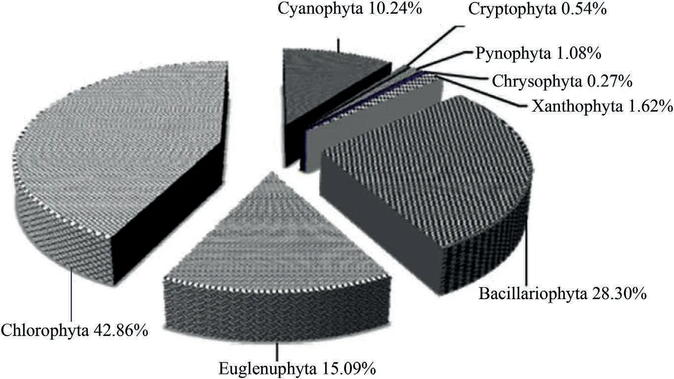
Fig. 2. The proportion of phytoplankton in the Backshore Wetland of Expo Garden Shanghai.

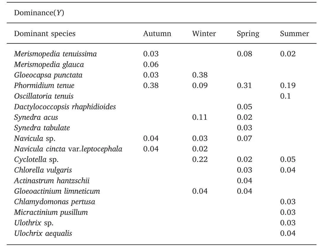
Table 3 Dominance of the dominant phytoplankton species in different seasons in the Backshore Wetland of Expo Garden Shanghai.

3.4. The abundance and biomass of phytoplankton

The average annual abundance of phytoplankton in the Backshore Wetland was 711.11 ± 1103.98×104cells/L (range:4.38×104-9407.97×104cells/L).The abundance of Cyanophyta was the highest with an annual average of 330.99 ± 350.63×104cells/L,or 47.74% of all cells. The second most abundant species was Bacillariophyta (184.24 ± 235.86×104cells/L),which accounted for 26.57%, while Chlorophyta was the third most abundant(168.02 ± 183.09×104cells/L, 24.23%). The seasonal variation of phytoplankton density showed a bimodal pattern (Fig. 3). The main peak appeared in winter (February), and the average density was 2291.64 ± 3290.86×104cells/L, and a secondary peak appeared in summer, being 1309.74 ± 835.76×104cells/L. The lowest was in autumn (September), 14.88 ± 10.92×104cells/L.

The average annual biomass of phytoplankton in the Backshore Wetland was 5.70 ± 12.85 mg/L (range: 0.01-84.54 mg/L).Bacillariophyta had the highest biomass with an annual average of 3.41 ± 4.76 mg/L, which accounted for 61.46%. Cyanophyta and Chlorophyta were lower than Bacillariophyta, with annual averages of 0.84 ± 0.95 mg/L (15.19%) and 0.69 ± 1.13 mg/L (12.34%), respectively.The seasonal variation of biomass was also bimodal(Fig.3),however,the trends of biomass and density were not the same due to a large difference in the fresh weight of the different phytoplankton species. The main peak appeared in winter (January), and the average biomass was 16.79 ± 22.22 mg/L, and a secondary peak appeared in summer (August), 10.38 ± 16.23 mg/L. The lowest was in autumn(September), 0.12 ± 0.21 mg/L.

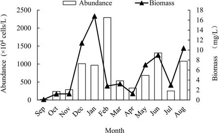
Fig. 3. Annual variation of abundance and biomass of phytoplankton in the Backshore Wetland of Expo Garden Shanghai.

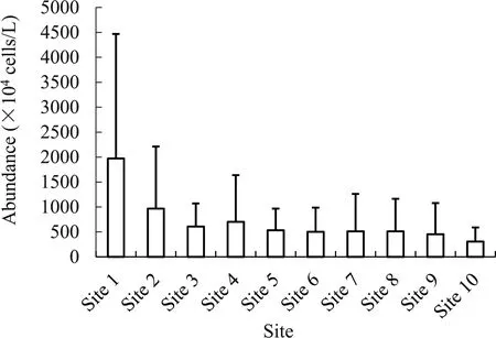
Fig. 4. Horizontal variation of phytoplankton abundance in the Backshore Wetland of Expo Garden Shanghai.

3.5. Spatial distribution of phytoplankton stock

The distribution of phytoplankton at the different sites is shown in Figs. 4 and 5. The highest abundance of phytoplankton was found in Site 1 (2496.91 ± 1971.29×104cells/L), accounting for 27.91% of the total abundance of phytoplankton. Site 2(1246.22 ± 966.36×104cells/L) was the second highest and accounted for 13.68%. The abundance of cells gradually decreased along the direction of water flow until Site 10(306.09 ± 283.84×104cells/L),where abundance was only 4.33%.The abundance of phytoplankton at Site 1 was 6.44 times that of Site 10.

Due to the predominance of diatoms which have larger individual fresh weights than others, the biomass of Site 4(28.30 ± 14.66 mg/L)reached a maximum and accounted for 26.04% of the total biomass.The biomass at Site 1 (18.91 ± 12.96 mg/L) was the second highest and accounted for 23.02%, and Site 10 (2.03 ± 1.62 mg/L) had the lowest biomass with only 3.61%. The biomass at Site 4 was 7.22 times that of Site 10.

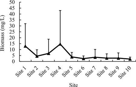
Fig. 5. Horizontal variation of phytoplankton biomass in the Backshore Wetland of Expo Garden Shanghai.

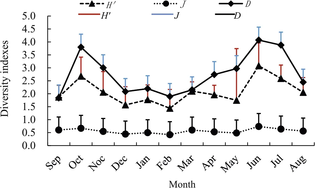
Fig.6. Month variation of diversity indexes of phytoplankton in the Backshore Wetland of Expo Garden Shanghai.

According to the statistical analysis,the abundance of the Site 1 was significantly different from those of the other sites (F=2.269,P=0.023). The difference between Site 2 and Site 10 was significant(P=0.033), while the differences between the other sites were not significant(P ＞0.05).The biomass at Site 4 was significantly different from those of Sites 5, 6, 7, 8, 9, and 10 (P ＜0.05). In addition, Site 1 was different from Site 6 and Site 10 (P ＜0.05).

3.6. Spatial and temporal patterns of phytoplankton diversity

The Shannon-Wiener diversity index(H′),Margalef species richness index (D) and Pielou's species evenness index (J) of the Backshore Wetland in the Shanghai World Expo Park fluctuated from 1.44 to 3.08,1.84 to 4.07, and 0.42 to 0.74, respectfully. Their average values were 2.08 ± 0.46, 2.74 ± 0.76, and 0.56 ± 0.09, respectfully. The three diversity indices showed an obvious seasonal variation trend,with high values in summer and autumn and low values in winter and spring(F=10.852, 13.447, 6.371, P ＜0.01) (Fig. 6). The maximum values for the three diversity indices occurred in June,the minimum values for the Shannon-Wiener diversity index (H′) and Pielou's species evenness index (J) occurred in February, and the minimum values for the Margalef species richness index (D) occurred in September.

In Fig. 7, the Shannon-Wiener diversity index (H′) and Pielou's species evenness index (J) were not significantly different at each site(F=0.398, 0.458, respectively, P ＞0.05, n=120), while the Margalef species richness index(D)at Site 1 was significantly different from that at Sites 5 and 10 (P=0.045, 0.032, respectively, n=120).

3.7. CCA analysis on the phytoplankton community and the environmental factors

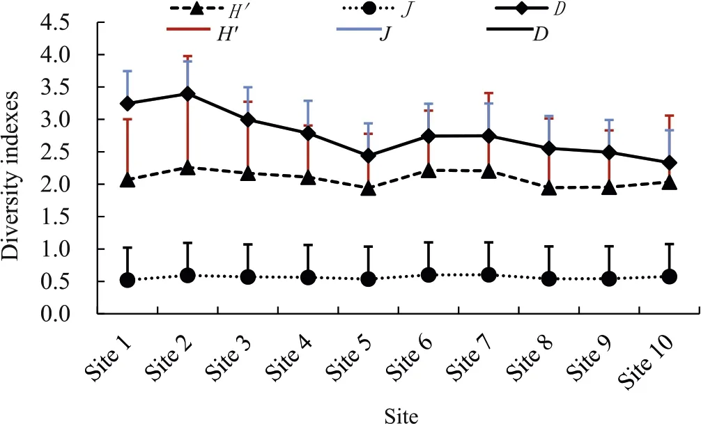
Fig. 7. Horizontal variation of diversity indexes of phytoplankton in the Backshore Wetland of Expo Garden Shanghai.

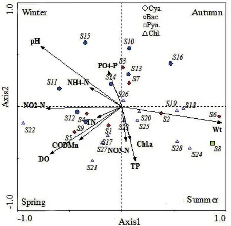
Fig.8. CCA biplot of phytoplankton species and environmental variables in the Backshore Wetland of Expo Garden Shanghai.

Based on phytoplankton relative abundance (≥0.2%) and the frequency of occurrence(≥32%),28 types of phytoplankton were selected for the CCA analysis.Fig.8 showed that the eigenvalues for the first and second sorting axes were 0.180 and 0.084,respectively.The correlation coefficients between the environmental factors and the ranking axis of the species were 0.931 and 0.794, respectively. This indicated that the result were reliable and accurately reflected the relationship between phytoplankton and environmental factors. The correlation coefficients between the environmental factors and the first two order axes were shown in Table 4.

Water temperature, pH, nitrites, and dissolved oxygen (DO) had higher correlation with 1st axis in the CCA biplot, whereas pH, water temperature, and TP showed higher correlation with the 2nd axis, indicating that temperature increased from left to right,and pH decreased from top to bottom.

According to the distribution characteristics of the 11 environmental factors,the CCA ordination analysis classified 28 phytoplankton species into 3 groups(Table 5 Phytoplankton Codes).The species Group I were spring species, which consisted mainly of Cyanophyta and Chlorophyta species. The distribution pattern was positively related to dissolved oxygen and nitrite nitrogen. The species Group II were summer species, which mainly consisted of Chlorophyta species, and the distribution patterns were positively correlated with watertemperature. The species Group III were autumn and winter species,which mainly consisted of Bacillariophyta species, and their distribution patterns had a negative correlation with water temperature and a positive correlation with pH.

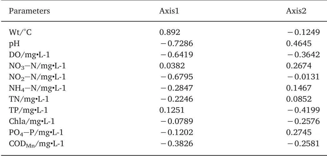
Table 4 Correlation coefficients between environmental factors and the first two or dination axes.

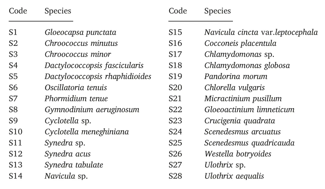
Table 5 Codes of phytoplankton species for CCA.

4. Discussion

4.1. Characteristics of phytoplankton community structure dynamics

The composition of phytoplankton species is a result of phytoplankton that adapt to their water environment (Reynolds, 2000, pp.123-132; Tan, Ma, & Liu, 2007; Li & Han, 2007). Therefore, different nutrient conditions inevitably lead to different compositions of algae and differences in dominant species, densities, and biomass. There are abundant phytoplankton species in the Expo Park beach wetland,where Chlorophyta, Bacillarriophyta, and cyanobacteria are the most dominant groups, consistent with the results of Hong and Chen (2002) regarding the aquatic communities of Chinese rivers since the 1950s.From the perspective of phytoplankton species composition, the Backshore Wetland has the general characteristics of a river.

Seasonal variation of the dominant phytoplankton species occurred throughout the year.There number of Cyanophyta and Euglenophyta in the warm season are higher than that in the cold season, because pigments of both phyla can withstand high temperatures and are suited for surviving on organic nutrients.During the warm season,organic matter is readily decomposed and cyanobacteria can multiply, which leads to the superiority of Phormidium tenue and Oscillatoria tenuis (Guo, Lin, &Li,1997).The number of diatoms in the warm season was less than the cold season because diatoms grow better at relatively low temperatures and cannot survive in high-temperature environments.The growth and breeding of diatoms are affected by many factors, such as water flow rate, water temperature, nutritional status, and other various water quality indicators. In general, pristine, hard water bodies at low temperature, with a moderate flow rate are better suited for diatoms.During the sampling at the Backshore Wetland in the Shanghai World Expo Park, the water temperature ranged from 2.9 to 21.6°C in winter and spring with high clarity. These conditions meet the growth requirements for diatoms, which then give diatoms an advantage in winter and spring over other species that are not as suited for those kinds of conditions, contributing to Cyclotella sp., Synedra acus, and Navicula sp. being the dominant species. In summary, the seasonal variation of phytoplankton abundance is obvious.The dominant taxa in May were diatoms and in June it was green algae.The dominant taxon was cyanobacteria from July to November, but the degree of cyanobacteria was weakened month by month. In December and January, it was replaced by diatoms again. Due to the large-scale reproduction of Synedra acus and Navircula sp. in February, diatoms became dominant taxa and their abundance reached a maximum.

4.2. Response of phytoplankton community structure to ecological restoration

The unity between an organism and its habitat is manifested in the relationship between the organism and its surrounding environment.Phytoplankton population structure and distribution are usually directly affected by the habitat (Lin, Tang, & Zhuang, 1994). Under ecological restoration, phytoplankton density showed a decreasing trend along the direction of water flow. Site 1 was 6.44 times that of Site 10.These differences are likely due to the environmental setting of the sites. Site 1 was located at the head of Backshore Wetland, and the water comes from the Huangpu River that is filtered through filter tank,and the N and P concentrations are higher at Site 1 than at the other sites.Studies have shown that a high concentration of nutrients,within a certain range, can promote an increase in phytoplankton density,which can contribute to an increased growth of phytoplankton (Qian,Wang,&Chen,2009).Site 1 is also close to clusters of aquatic plants in the Backshore Wetland, such as Hydrilla verticillata, Vallisneria natans,Potamogeton distinctus, Myriophyllum spicatum, Potamogeton crispus,Ceratophyllum demersum, and Elodea nuttallii (Zhan, Dong, & Jin, 2010,pp. 18-21). Aquatic plants can quickly absorb the nutrients in water bodies and sediments,which can reduce the available nutrients that are necessary for the growth and reproduction of phytoplankton. Aquatic plants can also secrete substances that inhibit the growth of phytoplankton. Lei (2008) showed that there are more N and organic matter in the sediments of a grass area,which transports N and organic carbon in water to the bottom of the mud, allowing them to enter the earth biochemical cycle. It effectively reduces the N concentration in the water and limits the nutrients that are used by phytoplankton for growth. The results of the prior study and our current study are consistent; that is, the number and density of phytoplankton species are significantly and positively correlated with nitrate nitrogen(F=0.395,P ＜0.01; F=0.225, P=0.018). Zhang, Chen, He, Wu, and N (2007)showed that Hydrilla verticillata, Ceratophyllum demersum, and others have a strong inhibitory effect on the growth of Chlorella pyrenoidosa and Scenedesmus obliquus. All of the tested plants had different degrees of an algae control effect and could effectively promote sludge deposition and inhibit the resuspension of bottom sediments. This causes the abundance of phytoplankton to be greatly reduced when there is a double effect caused by a decrease in nutrient salt concentration and the control of algae by large aquatic plants. Therefore, phytoplankton density at Site 10 was the lowest.

4.3. Effect of environmental factors on the community structure

The environmental factors that caused changes in the phytoplankton community structure included nutrient status, temperature,light, and pH. Phytoplankton species may vary under different environmental conditions, such as the distribution of stain-resistant species in eutrophic or organic-rich water bodies or the distribution of oligosaccharides in more pristine and transparent water bodies (Buzzi,2002; Mohan et al., 2007; Sladecek, 1983). Therefore, the main environmental factors that affect a phytoplankton community depend on location. Habib, Tippett, and Murphy (1997) pointed out that temperature, dissolved oxygen, transparency, and chemical oxygen consumption have the greatest impact on phytoplankton communities.

CCA analysis showed that water temperature, nitrite nitrogen, pH,and total phosphorus were the main factors that influence distribution of phytoplankton. Reynolds (1984) indicated that temperature is usually the most limiting and direct environmental factor that affects phytoplankton growth. A CCA biplot of the main species and environmental variables also showed that water temperature was one of the most important factors that affected the abundance and distribution of phytoplankton in the wetland.In winter(February),the 1st distribution peak appeared as Synedra acus, Navircula sp. and Navicula cincta var.leptocephala became the dominant species. The 2nd peak occurred in June as the temperature increased and Gymnodinium aeruginosum,Chroococcus minutus, and Scenedesmus arcuatus became the dominant species. CCA analysis showed that blue-green algae had a significant and positive correlation with water temperature; moreover, S24, S28,and S6,especially, had intersections at the vertical line and the habitat factor line closest to the arrow, and so they were the most affected by temperature.However,in this study,only the number of phytoplankton species and water temperature reached a very significant and positive correlation (F=0.368, P ＜0.001), but density and biomass did not significantly correlate with water temperature (F=0.0.109, -0.090,respectively;P ＞0.05).This may be due to the fact that the dominant phytoplankton species each month was not the same for a single site and that different species have different optimal temperature ranges with different correlations corresponding to seasonal and water temperature changes.

Nutrients facilitate the survival of phytoplankton. Home and Goldman (1994) showed that phosphorus is a limiting factor for algal growth when the weight ratio of nitrogen to phosphorus is greater than 10. The annual average TN/TP of the Backshore Wetland is 53.97,which greatly exceeds this threshold.Therefore,TP is the main limiting nutrient for the growth and reproduction of phytoplankton in the Backshore Wetland. Chlorophyll-a is a comprehensive indicator that reflects the biomass of phytoplankton in the water. The Pearson correlation analysis confirmed a significant and positive correlation between chlorophyll-a and TP (F=0.422, P ＜0.01). In addition, the CCA analysis showed that most blue-green algae had a positive correlation with TP.

5. Conclusions

This study improves our understanding of phytoplankton dynamics in the Backshore Wetland. The annual variation of phytoplankton community structure and species diversity was examined for the Backshore Wetland of Expo Garden in Shanghai from September 2009 to August 2010. The results showed that the number of Chlorophyta species were the most abundant, followed by diatoms. The seasonal trend of existing stocks was bimodal, with main peaks of density and biomass occurring in the winter and a secondary peak occurring in the summer. Phytoplankton abundance gradually decreased from site 1 to site 10 along the direction of water flow.The Shannon-Wiener diversity index(H′),the Margalef species richness index(D),and Pielou's species evenness index(J)all showed a clear seasonal trend.All indices showed a changing pattern, with the highest recorded values from the summer to autumn and the lowest recorded values from the winter to spring.

Phormidium tenue, Erismopedia tenuissima, Cyclotella sp., Navicula sp.,Gloeocapsa punctata, Navicula cincta var. Leptocephala, Synedra acus,Gloeoactinium limneticum, and Chlorella vulgaris were the dominant species in the study area. Through the study of phytoplankton community changes, the background and evolving trends of phytoplankton species in this area can be evaluated, providing basic data for studying regional water environmental quality and ecosystem change research.