Charney’s Model—the Renowned Prototype of Baroclinic Instability—Is Barotropically Unstable As Well

Yuan-Bing ZHAO and X.San LIANG∗,2,3

1School of Atmospheric Sciences,Nanjing University of Information Scienceand Technology,Nanjing 210044,China

2School of Marine Sciences,Nanjing University of Information Science and Technology,Nanjing 210044,China 3School of Mathematics and Statistics,Nanjing University of Information Science and Technology,Nanjing 210044,China

ABSTRACT The Charney model is reexamined using a new mathematical tool,the multiscale window transform(MWT),and the MWT-based localized multiscaleenergeticsanalysisdeveloped by Liangand Robinsontodeal with realistic geophysical f luid f low processes.Traditionally,though this model has been taken as a prototype of baroclinic instability,it actually undergoes a mixed one.While baroclinic instability explains the bottom-trapped feature of the perturbation,the second extreme center in theperturbation f ield can only beexplained by anew barotropic instability when the Charney–Green numberγ1,which takes place throughout the f luid column,and is maximized at a height where its baroclinic counterpart stops functioning.The giving way of the baroclinic instability to a barotropic one at this height corresponds well to the rectif ication of the tilting found on the maps of perturbation velocity and pressure.Also established in this study is the relative importance of barotropic instability to baroclinic instability in terms ofγ.Whenγ1,barotropic instability is negligible and hence the system can beviewed aspurely baroclinic;whenγ1,however,barotropic and baroclinic instabilitiesareof thesameorder;in fact,barotropic instability can beeven stronger.Theimplication of theseresultshasbeen discussed in linking them to real atmospheric processes.

Key words:Charney’s model,multiscale window transform,canonical transfer,baroclinic instability,barotropic instability

1.Introduction

The Charney model(Charney,1947)as a prototype of baroclinic instability has been extensively studied.The resulting perturbation patterns,though idealized,havebeenutilized to interpret the generation of midlatitude synoptic disturbances,such asthosein frontal dynamics,storm track dynamics(e.g.,Blackmon et al.,1977;Hoskins and Valdes,1990;Nakamura,1992;Chang and Orlanski,1993),and so forth.Even today,this seemingly very old f ield is still active(Badin,2014;Chai and Vallis,2014).As noted by Pierrehumbert and Swanson(1995),“Baroclinic instability is far from aclosed book,even in very classic areas.”Indeed,there are still questions unanswered with this model.For instance,though most of the perturbation f ields for an unstable mode are bottom-trapped,the vertical perturbation velocity wis not,and,moreover,there exists a second extreme on the sectional distributions of the zonal perturbation f low uand perturbation temperature T(refer to section 3.3 in this study).How is this secondary center of the perturbation generated,and whereisitsenergy from,if,in theclassical point of view,thesystem undergoesabottom-trapped baroclinic instability?

The only relevant explanation of the upper secondary maximum so far may comefrom theisentropic potential vorticity(PV)perspective.In the Charney model,the eastward propagating surface Rossby wave interacts with an internal Rossby wave,which liveson thebackground PV gradientand travelswestward relativeto thef low.Thephasesof thesetwo counter-propagating Rossby wavesmust lock for exponential growth(Hoskins et al.,1985).Such an explanation is intuitive,but,morefundamentally,what behind theinteraction is still unclear.A question f irst coming into mind is:how are the Rossby wavesgenerated beforetheinteraction,and where do thetwo wavesreceiveenergy for their growth?

On theother hand,it haslong been overlooked that Charney’s model admitsinstability processes that are local in nature.We know that,in the model,the interior PV gradient¯qyispositive,and so is the vertical shear at the lower boundary.Thismeetsoneof the four Charney–Stern–Pedlosky instability conditions(e.g.,Vallis,2006).However,such acondition is stated in a global sense,which does not imply a local instability structure.With regards to the Charney model,one often seestilting patternson thesectional distributionsof perturbation f ields.The westward tilting of the phase lines with heightonthedistributionsof uand p(seesection3.3below)isan indicator of baroclinic instability by theclassical result.However,thephasevariation with height isconf ined near the bottom.Over mostof thef luid column thephaselineisnearly straight(e.g.,Charney,1947;Kuo,1952,1979;Green,1960;Geisler and Garcia,1977;Fullmer,1982;Branscome,1983).Consequently,theheatf lux viatheunstablewavewill besimilarly conf ined to aregion near thelower boundary.

Historically,multiscaleenergeticsanalysishasbeen used to infer the instability characteristics of the Charney model,sinceinstabilitiesareessentially energy transfer processesbetween the mean and perturbation f ields.Kuo(1952)argued that,in the Charney model,downward transport of zonal momentum uwand northward heat transport vTare important energy sources for perturbation kinetic energy.However,other studies(e.g.,Green,1960,1970;Fullmer,1982;Branscome,1983;Pedlosky,1987)have shown that the perturbation energy source in the Charney model is the potential energy(from the sloping isentropic surfaces)rather than the kinetic energy release of the vertical shear of the basic f low.On the other hand,although some of these features in the Charney model agree with those of more realistic atmosphere,major discrepancies exist between results derived from linear theory and observations.For instance,in the Charney model perturbation energy has only one maximum at the surface(Charney,1947;Brown,1969;Song,1971;Simons,1972),whereas in the real atmosphere there are two maxima in the vertical,one at the surface and the other near the tropopause,and the latter is in fact larger(e.g.,Kao and Taylor,1964;Lorenz,1967).In some studies the formation of theupper-level maximum hasbeen investigated with more realistic models(e.g.,Simons,1972;Gall,1976a;Simmons and Hoskins,1978),but few studieshaveever been dedicated to explaining the secondary maximum at the upper levels of the Charney model.Onepossiblereason may bebecausethe maximum isunrealistically weak,whilst another may be due to the limitation of the methods available then.The above questions,though with ahighly idealized model,actually appear to be di f fi cult.Thedi f fi culty comesfrom themultiscale energetics,which form convenient diagnostic quantities for theproblem,butdo nothavetheneeded local structurewithin the classical framework.

Ever since Lorenz(1955)set up a two-scale formalism of energetics with the Reynolds decomposition,energetic analysis has become a powerful diagnostic tool for dynamic meteorology.This has been seen previously in studies of mean f low–wave/eddy interaction(e.g.,Dickinson,1969;Fels and Lindzen,1973;Boyd,1976;McWilliams and Restrepo,1999),atmospheric blocking(Trenberth,1986;Fournier,2002),regional cyclogenesis(Caiand Mak,1990),and storm tracks(e.g.,Chang and Orlanski,1993;Chapman et al.,2015),to name a few.This tool is particularly useful for thepurposeof thisstudy becausetheinstability of abackground f low isessentially aprocessthattransfersenergy from the background to perturbations.However,classical energetics,and the Lorenz cycle in particular,are stated in global form.That is to say,they are expressed in global averagesor integrals(e.g.,Pedlosky,1987).In the past several decades,there has been a continuing e f f ort to relax the spatial averaging/integration in order to extend this global formalism to regional atmospheric processes,for which averaged energetics may not yield useful information because of their localized nature(they tend to belocally def ined in spaceand time and can be on the move).The instability that we will look in this study is such an example;it obviously has a vertical structure which will be disguised in a mean quantity diagnosis.The extension,of course,is by no means as trivial as a relaxation of the averaging/integration.The major issue here is how to separate the in-scale transport and the cross-scale transfer from the intertwined nonlinear process.A tradition started by Lorenz himself isto collectthetermsin divergence form,and takethem astherepresentation of thetransportprocess.The remainder of the nonlinear interaction is then the energy transfer between thedistinct scales(e.g.,Harrisonand Robinson,1978).

The above approach to separating transport and transfer processes has been a standard practice in f luid dynamics research,particularly in turbulence research(cf.Pope,2000).However,there is a severe issue to be resolved,as long pointed out by Holopainen(1978)and Plumb(1983)but mostly overlooked.While it is known that a transport process indeed bears a divergence form in the governing equations,theseparation isnotunique.Multipledivergenceforms exist that may yield quite di f f erent transfers;that is to say,the so-obtained energy transfer in such an open system is quite ambiguous.This issue,which is actually quite profound in f luid dynamics,has long been identif ied but has not received enough attention,except for a few studies such as Plumb(1983).An early attempt to solve this problem is the multiscaleenergeticsanalysisby Liangand Robinson(2005),whichisbased onthemultiscalewindow transform(MWT),a functional analysistool thatwaslater on rigorized(Liang and Anderson,2007).However,in Liang and Robinson(2005),the transport–transfer separation was introduced in a halfempirical way.Recently,Liang(2016)found that this actually can be put on a rigorous footing.The energy transfer can be rigorously derived,and theresulting expression is unique.Moreover,it bearsa Liebracket form,reminiscent of the Poisson bracket in Hamiltonian mechanics.In this study,we use the MWT-based multiscale energetics method to reexaminethe Charney model and,unexpectedly,f ind that this model,which has been taken as a prototype of baroclinic instability,actually undergoesamixed one;thesecond extreme center on the perturbation f low can be largely explained by the newly discovered barotropic instability,and the accompanied kinetic energy(or barotropic)transfer is mainly contributed from the vertical momentum f lux.

The paper is organized as follows:In the next two sections,we brief ly introduce the methodology and the Charney model.Followed isadescription of thegeneration of the dataset needed for thestudy.In section 4,adetailed energeticsanalysisispresented.Thiswork issummarized in section 5.

2.Localized multiscale energy and vorticity analysis

The research method for this study is the multiscale energetics part of the localized multiscale energy and vorticity analysis,or MS-EVA for short(cf.Liang and Robinson,2005);also to be used is the MS-EVA-based theory of localized f inite-amplitude baroclinic and barotropic instabilities(Liang and Robinson,2007).Thisisasystematic lineof work,involving ingredientsfrom di f f erentdisciplinessuch as mathematics and geophysical f luid dynamics.A comprehensive description is beyond the scope of this paper.In the followingwepresentjustavery brief introduction.Thereader is referred to Liang(2016)for details,or,alternatively,to Liang and Wang(2018),section 2,for another short introduction but with more detailsfurnished.

MS-EVA is based on a novel functional analysis tool called multiscale window transform(MWT;Liang and Anderson,2007).With the MWT,onecan split afunction space into a direct sum of several mutually orthogonal subspaces,each with an exclusive range of time scales,while having its local propertiespreserved.Such asubspaceistermed a“scale window”,or simply a“window”.A scalewindow isbounded aboveand below by two scalelevels.In the M-window case,they are bounded above by M scale levels:j0,j1,...,jM−1.(A level j corresponds to a period 2−jτfor a time duration τ.)For convenience,these windows will be denoted with=0,1,...,M−1,respectively.

MWT can be viewed as a generalization of the classical Reynolds decomposition;originally it was developed to faithfully represent the energies(and any quadratic quantities)on the resulting scale windows.This is the key to multiscale energetics analysis.Liang and Anderson(2007)found that,for some specially constructed orthogonal f ilters,there exists a transfer-reconstruction pair,namely,MWT and its counterpart,multiscale window reconstruction(MWR),just like Fourier transform and inverse Fourier transform.In other words,MWRisjust likeaf ilter in thetraditional sense.What makes it distinctly di f f erent is that,for each MWR,there exists an MWT which gives transform coe f fi cients that can be used to represent the energy of the f iltered series.(Normally,with a traditional f ilter there are no such coe f fi cients and hence energy cannot even be represented;see below).

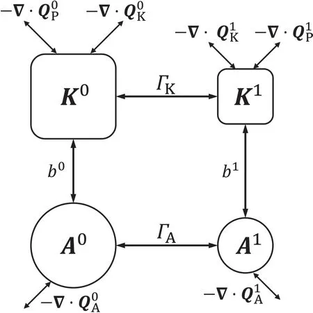
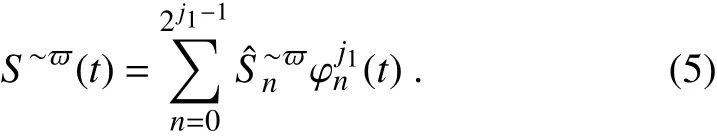
Fig.1.Schematic illustration of the MS-EVA energetics for a two-scale window decomposition.The symbols are conventional in MS-EVA studies,withthesuperscripts0 and 1signifying the time-mean and perturbation windows,respectively.See Eqs.(8)and(9)and Table 1 for interpretations of the symbols.

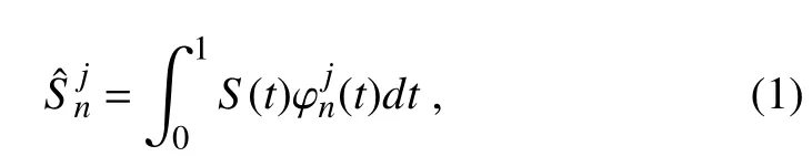
Now,suppose{ϕjn(t)}nis an orthonormal translational invariant scaling sequence[built from cubic splines;see Liang and Anderson(2007)and Fig.1in Liang(2016)],with j some scalelevel,n thetimestep,and t thetimevariable.Let S(t)be some square integrable function def ined on[0,1](if not,the domain can always be rescaled to[0,1]).Liang and Anderson(2007)showed that,in practice,all such functionscan be expanded with{ϕjn(t)}nasabasis;and theresulting transform,

for any scalelevel j(corresponding to frequency 2j),iscalled a scaling transform.Given window bounds j0,j1for a twowindow decomposition,S can then be reconstructed on the windowsformed above:

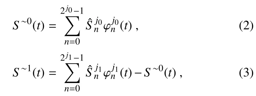
where∼0,∼1 indicate the corresponding scale windows.With these MWRs,the MWTof S isdef ined as

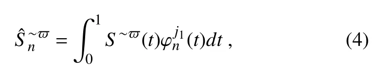
for windows=0,1 and n=0,1,···,2j1−1.In termsofthe above MWRs can bewritten in oneequation:

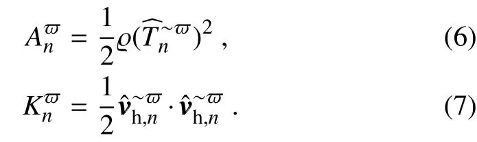
With MWT,the available potential energy(APE)and kinetic energy(KE)densities(for convenience,wesimply refer to them as APEand KE,unlessconfusionmay arise)for windowcan bedef ined,following Lorenz(1955),as

In the above def initions,vvvh=(u,v)is the horizontal velocity,T is the temperature anomaly[with the mean vertical prof ile T(z)removed],andis a proportionality depending on the buoyancy frequency.In the absence of di f f usion/dissipation,the multiscale energy equations for a geophysical f luid system can now be symbolically written out(location n in the subscript omitted henceforth for simplicity):

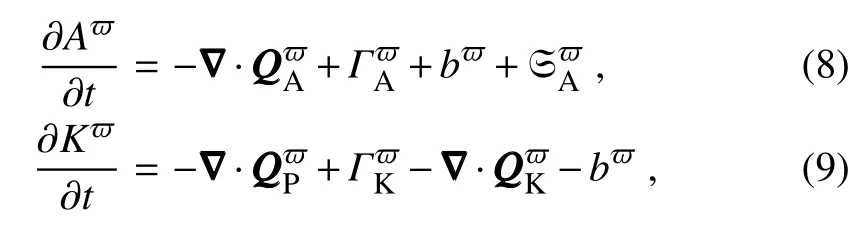
for=0,1.The mathematical expressions and interpretations of the terms in Eqs.(8)and(9)are tabulated in Table 1;their names are the same as many others(e.g.,Orlanski and Katzfey,1991;Chang,1993;Yin,2002)aNotethat thetimetendency in Eqs.(8)and(9)in Charney’s model is meaningless since thebasic f low has been assumed to besteady.Nevertheless,it has nothing to do with theother termsin theenergy equation,in which weareinterested most..It should be noted that all terms are localized both in space and in time;in other words,they are all four-dimensional f ield variables,distinguished notably from theclassical formalismsin which localization is lost in at least one dimension of space–time to achievethescaledecomposition.Processesintermittent in space and time are thus naturally embedded in Eqs.(8)and(9).Figure 1 schematizes the local Lorenz cycle with a twowindow decomposition.

Although thetermsin Eqs.(8)and(9)havethetraditional names,they are distinctly di f f erent from those in the traditional formalism.The most distinct terms areΓandΓ.For a scalar f ield S within a f low vvv=(u,v,w),the energy transfer from other scale windows to windowrigorously proves(Liang,2016)to be(now the subscript n issupplied)

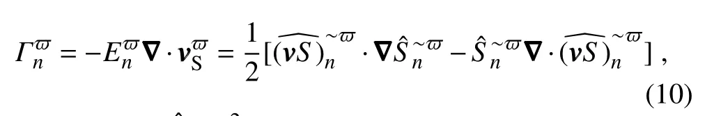
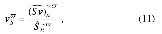
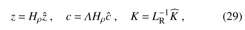
is referred to as the S-coupled velocity.According to Eq.(10),Γnhasa Liebracket form,reminding usof the Poisson bracket in Hamiltonian mechanics[arecent referencelinking geophysical f luid dynamics(GFD)to Hamiltonian mechanics isreferred to Badin and Crisciani(2018)].It also possessesa very important property,

as f irst proposed in Liang and Robinson(2005)and later proved in Liang(2016).Physically,thisimpliesthatthetransfer is a mere redistribution of energy among the scale windows,without generating or destroying energy as a whole.Thisproperty,though simpleto state,doesnot hold in previousenergetic formalisms(see below for acomparison to the classical formalism).To distinguish it from those that may have been encountered in the literature,it is termed“canonical transfer”.

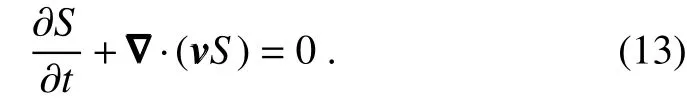
Canonical transfer is fundamentally associated with energy conservation among scalewindowsduring nonlinear interactions;this forms the key of themode–mode interaction.That is to say,a mode may receive energy or lose energy to another mode,but on the whole energy should be conserved,asstated by Eq.(12).To further illustratehow canonical transfer di f f ers from the classical formalism,in the following we consider aspecial case,i.e.,a case with the traditional Reynolds decomposition.Since by Liang and Anderson(2007),MWTisageneralization of the Reynoldsdecomposition(i.e.,themean-eddy decomposition),wecan specializeto consider thismost particular case.Now,consider apassivetracer S in an incompressiblef low,and neglect di f f usion for simplicity:

Perform a Reynolds decomposition S=

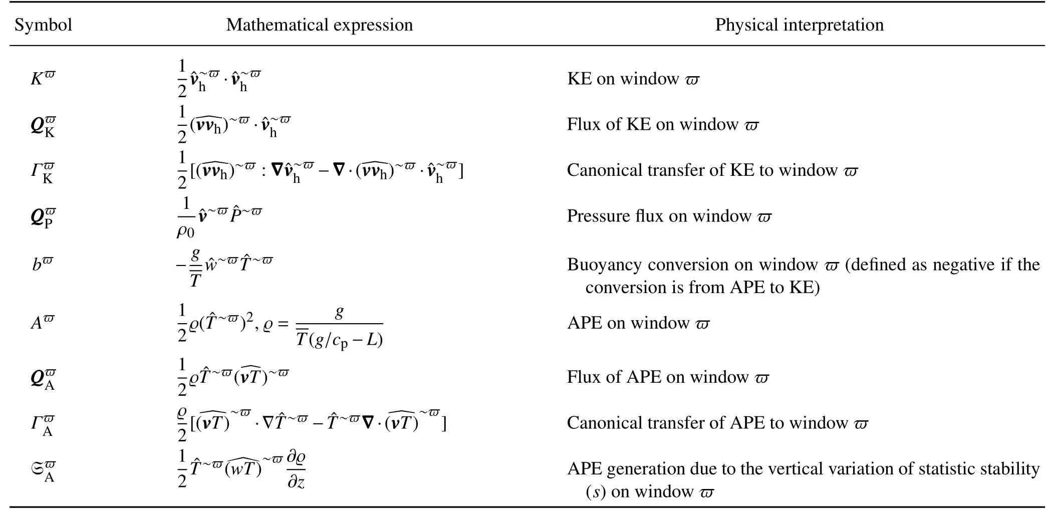
Table 1.Mathematical expressions and physical interpretations for the energetics terms in Eqs.(8)and(9).The colon operator(:)inΓK andΓA isdef ined such that,for two dyadic products AAABBB and CCCDDD,(AAABBB):(CCCDDD)=(AAA·CCC)(BBB·DDD).For details,refer to Liang(2016).

the termsin divergenceform are generally understood asthe transports of the mean and eddy energies,and those on the right-hand side as the respective energy transfers.The latter are usually used to explain the dynamical source of the mean f low–eddy interaction.Particularly,when S is a velocity component,the right-hand side of the eddy energy equation,R=−hasbeeninterpreted astherateof energy extracted by Reynoldsstress,or“Reynoldsstressextraction”for short,against the mean f ield to fuel the eddy growth;in the context of turbulence research,it is also referred to as the“rate of the turbulence production”(Pope,2000).It has also been extensively utilized in dynamic meteorology to explain phenomena such as cyclogenesis,eddy shedding,etc.However,Holopainen(1978)and Plumb(1983)found that the transport-transfer separation is not unique and hence the resulting transfer seems to be ambiguous.Moreover,the two energy equationsdo not,in general,sum to zero on therighthand side.This is not what one would expect of an energy transfer,which by physical intuition should be a redistribution of energy among scalewindows,and should notgenerate nor destroy energy as awhole.

With the MS-EVA formalism,these are not issues any more.In thisspecial case,theenergy equationsin theformof Eqs.(8)or(9)become[see Liang(2016)for rigorousderivation;for a brief illustration,refer to the second section of Liang and Wang(2018)]

where

This is in sharp contrast to the traditional one:now,one can see that the right-hand side is balanced.ThisΓis the“canonical transfer”in this special case.Previously,Liang and Robinson(2007)illustrated,for a benchmark hydrodynamic instability model(Kuo,1949)whose instability structureisanalytically known,thetraditional Reynoldsstressextraction R doesnotgivethecorrectsourceof instability,while Γdoes.We further remark that these equations result from the MWT-based multiscale energetics formalism,which are rigorously derived through reconstructing atom-like building blocks of multiscale transports[see Liang(2016)];and they are unique.More specif ically,if S is temperature T,thenΓ isbaroclinic canonical transfer(ΓA),

witha multiplier depending on the lapse rate(see Table 1);if S is velocity(say u or v),Γis barotropic canonical transfer(ΓK).With a background f ield

From thisformula,it can clearly be seen that,within astratif ied baroclinic f low(as in the Charney model),perturbations can also extract kinetic energy from the vertical shear of the basic f low.

It has been established that the canonical transfer termsandΓK)in Eqs.(8)and(9)are very important.Particularly,themean-to-eddy partsof them correspond precisely to thetwo importantgeophysical f luid f low processes,i.e.,baroclinic instability and barotropic instability(Liang and Robinson,2007);detailsarereferred to arecent publication(Liang,2016).For notational convenience,they arewritten as BCand BT,respectively.A set of criteria was then derived in Liang and Robinson(2007)for instability identif ication:

(1)A f low is locally unstable if BC+BT>0,and vice versa;

(2)For an unstable system,if BT>0 and BC0,the instability thesystem undergoesisbarotropic;

(3)For an unstable system,if BC>0 and BC0,then the instability is baroclinic;and

(4)If both BT and BC are positive,the system must be undergoing amixed instability.

Because of their physical meanings,in the following we refer to BT and BC as barotropic transfer and baroclinic transfer,respectively.

We remark that the concept of barotropic and baroclinic instabilities here is in the classical sense(e.g.,Pedlosky,1987):a f low is baroclinically(barotropically)unstable if potential(kinetic)energy is the only form of energy transferred from the mean f low to perturbation f ields.However,the energy transfer terms used to infer instabilities,as denoted by BC and BT,are di f f erent from the traditional ones.In Eq.(7b),on spatial integration the f irst term(in a divergence form)on the right-hand side vanishes,whereas the second term−·does not.The second term can be further divided into two parts:−and−uw∂¯u/∂z.In the case of quasi-geostrophic f low,because w vanishes to the f irst order,the kinetic energy transfer related to the vertical shear,−uw∂¯u/∂z,is zero.(In fact,because of this,barotropic instability isconventionally believed to berelated only to the horizontal shear of the mean f low).But,it cannot betotally ignored.When localized instability isconsidered,it may appear signif icant locally,though globally it is still very small.Moreover,in some limiting cases,it could be signif icant.Theseareindeed what wewill f ind soon in the Charney model(seebelow).

3.A brief review of the Charney model

3.1.Basic state

The Charney model talks about the instability of a constant shear f low in a stratif ied,semi-inf inite atmosphere on aβ-plane to quasi-geostrophic perturbations.The mean state(denoted by an overbar)of the Charney model therefore assumes

whereΛis a constant.The mean temperature f ield(and mean density(¯ρ)aredetermined by thethermal wind relation

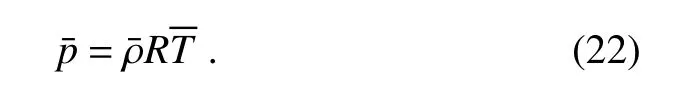
WithT andρ¯,themean pressurefe ild(p¯)isobtained accordngly by theequation of state

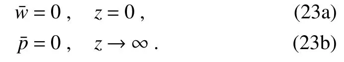
Thedomain of the Charney model issemi-inf initewith asolid f latbottom boundary.Theboundary conditionsare,therefore,

3.2. Eigenvalueproblem

Charney’s problem of baroclinic instability is governed by the linearized quasi-geostrophic PV equation(e.g.,Charney,1947;Kuo,1952;Green,1960;Burger,1962;Miles,1964;Lindzen and Farrell,1980)

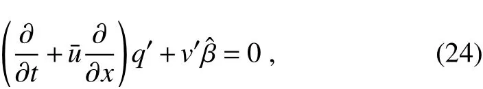
where qis the perturbation PV andˆβ=¯qyis the meridional gradient of thebackground PV:

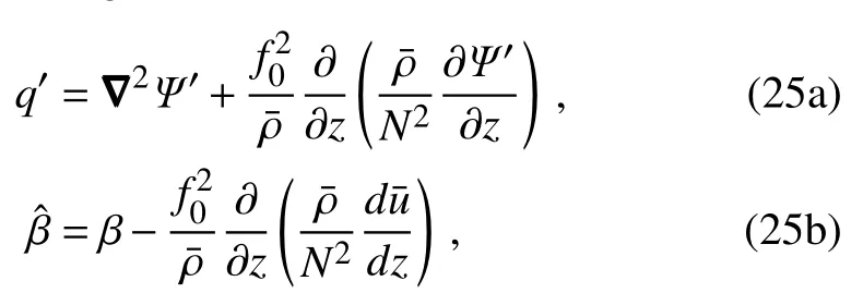
with f0the Coriolis parameter at a f ixed latitude,β=fy,Ψ,theperturbation streamfunction,and othersareconventional.In the Charney model,theabovetwo equationsaresimplif ied by assuming the buoyancy frequency N to be constant and¯ρ=ρ0e−z/Hρ,with Hρbeing a density scale height,which is also a constant.Under these assumptions,Eqs.(25a)and(25b)can besimplif ied as

Theboundary conditionsare w=0 at theground,i.e.,

and

Following convention,we look for normal modal solutionsof theform

where k and l are respectively the zonal and meridional wavenumber,and c is the complex phase velocity.Substitution of Eq.(27)into Eqs.(24)and(26)gives

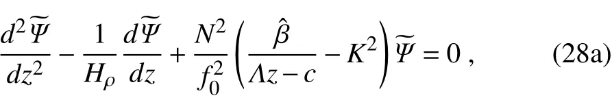
where K2=k2+l2,and

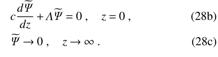
Theseequationsform an eigenvalueproblem.Since Eq.(28a)has a non-constant coe f fi cient,its analytical solution is not easy to obtain,but can be solved conveniently through numerical method.

Asin Chaiand Vallis(2014),wef irst non-dimensionalize Eqs.(28a)–(28c)using

where hats denote nondimensional quantities,and the horizontal scale is the Rossby radius def ined as LR=(NHρ)/f0.Equations(28a)–(28c)then become

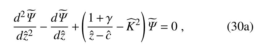
whereγ=(βL2R)/(HρΛ),and

The nondimensional parameterγin Eq.(30a)is known as the Charney–Green number.It isthe ratio of thescaleheight of the atmosphere Hρto the dynamic vertical scale h=(f20Λ)/(βN2)(Held,1978).As we can see,all the information on the mean f low(shear,stratif ication,latitude,etc.)is absorbed into this single parameter.Whenγ1,the solution corresponds to the deep mode;whereas,whenγ1,the solution approaches the shallow mode(e.g.,Held,1978;Branscome,1983).

In this study,we restrict ourselves to midlatitude(say 45◦N)waves,with f0andβf ixed.The vertical shearΛis independent of Hρand N,whereasthelatter two parametersare associated with each other through the thermal wind relation[Eq.(21)]and the equation of state[Eq.(22)].For instance,when Hρ=8800 m,N is about 0.0138.That is to say,γis only determined by two parameters,(Hρ,Λ)or(Hρ,N).Here,we use HρandΛ.Figure 2 shows the relation between Hρand N,and the distribution ofγon the(Hρ,Λ)-plane.We see that thelarger the Hρ,the smaller the N;and,if Hρisf ixed,γ increasesasΛdecreases,and viceversa.For convenience,we f ix the scale height Hρand letΛvary in order to investigate theinf luenceofγon the energetics.In thisstudy,we choose Hρ=8800 m(other values,e.g.,8200 m and 9400 m,have also been checked,and the results are similar).

We remark that Nakamura(1992)has once discussed the e f f ect of vertical shear on the structure of baroclinic waves.But the conclusion of this study is quite di f f erent from that of Nakamura(1992).According to Nakamura(1992),the vertical scale of baroclinic waves is inversely proportional to the vertical shear of the wind speed:h≈f Lx/(2πHowever,in the Charney model,both the vertical scale h and the wavelength Lxof the most unstable baroclinic wave are proportional to the vertical shear:h=f2∂¯u/∂z/(βN2)and Lx=f∂¯u/∂z/(βN)=Nh/f(Green,1960;Held,1978;Branscome,1983).This means that stronger vertical shear corresponds to longer and deeper waves,as opposed to theconclusion of Nakamura(1992).

3.3.Most unstablemodal solution

Without losing generality,letthemeridional wavenumber l=0.The most unstable mode therefore does not vary with y(e.g.,Lindzen and Farrell,1980).Theoretically,the model height is inf inite.In practice,it is set to be f inite but with enough high altitude(50Hρin this study).Discretize Eqs.(30a)–(30c)in the vertical direction,and the resulting eigenvalueproblem issolved through iteration.

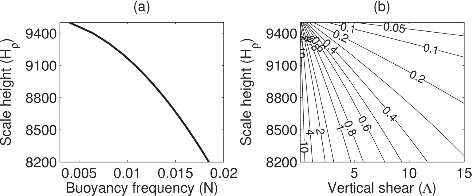
Fig.2.(a)The relation between scale height Hρ(meter)and buoyancy frequency N(s−1).(b)Distribution of the Charney–Green number on the(Hρ,Λ)-plane,whereΛisthevertical shear(10−3 s−1).

Figure 3 shows the variations of the nondimensional wavenumber,growth rate and phase speed of the most unstable mode withγ.We see that the wavenumber increases withγ,whereas the growth rate and phase speed decrease withγ.[Note that the nondimensional maximum growth rate doesnot decreasemonotonically,and it peaksatγ=0.4(Fig.3b).But its dimensional counterpart[multiplied by(f0Λ)/N)is monotonically decreasing withγ].This implies that a smallerγcorrespondsto longer and deeper waveswith larger growth ratesand faster phasespeeds.In particular,whenγ=1.33,thenondimensional wavenumberˆk of themost unstable mode is 1.4,corresponding to the dimensional wavenumber k=1.4×10−6m−1and wavelength L=4504km.And thecorrespondingnondimensional and dimensional growthratesare 0.3168 and 0.0175 hr−1,respectively,implying that thewave amplitude will double in 40 hours.These results are consistent with previous studies,such as Kuo(1952,1979),Gall(1976b),Lindzen and Farrell(1980),Farrell(1982),Chaiand Vallis(2014),to nameafew.

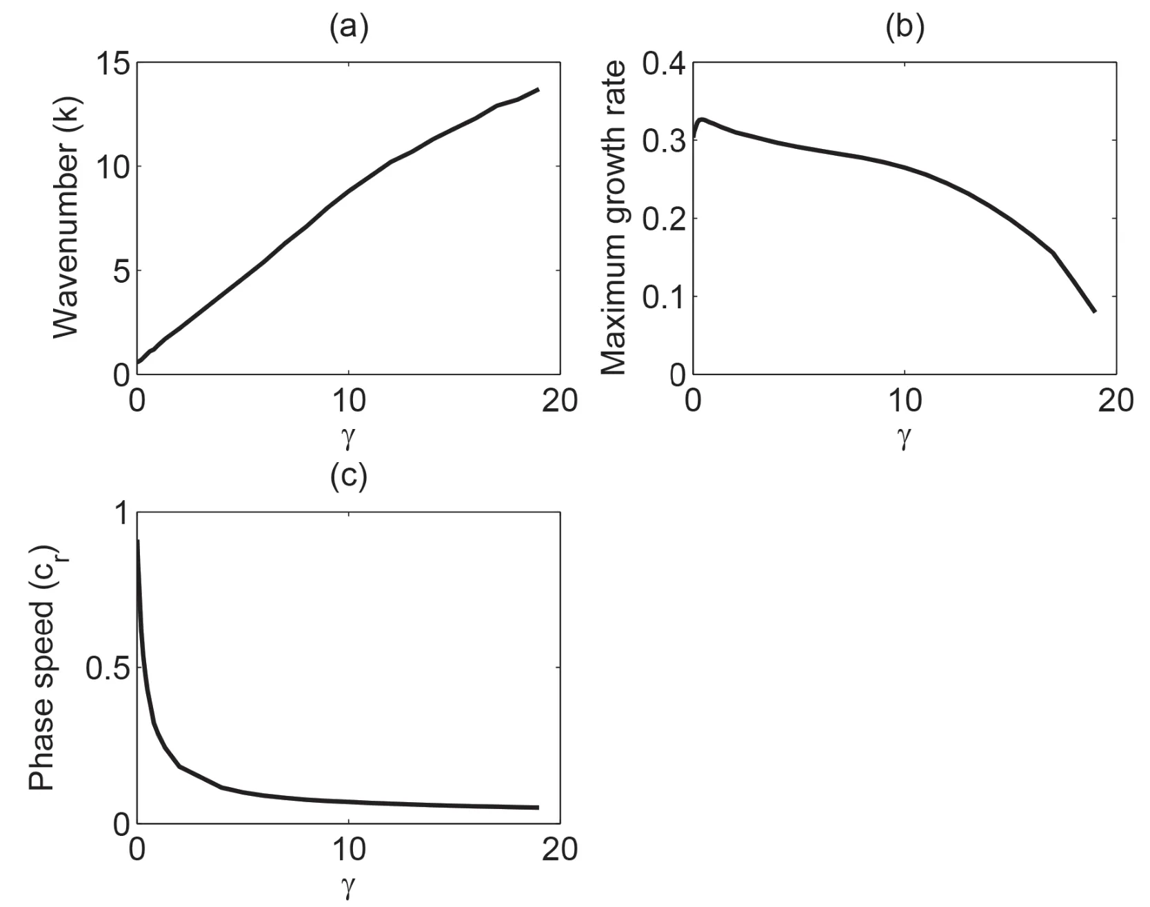
Fig.3.Nondimensional(a)wavenumber(k),(b)maximum growth rate,and(c)phase speed(c r)of the most unstablemodeasafunction of the Charney–Green number.

The perturbation f ields of pressure,velocity and temperature are required,the solutions of which can be found from the literature(e.g.,Kuo,1952;Charney and Drazin,1961;Gill,1982).In nondimensional form,they are given by,respectively,

and

SinceΨ,theeigenvector,isalready known,all theperturbation f ields can now be determined.

The computed perturbation f ields for the most unstable modeareshown in Fig.4.Here,weshow threetypical cases:two extreme cases(the deep modeγ=0.1 and the shallow modeγ=10),and onemoderatecase(γ=1).Wecan seethat the wave structure varies withγ.Firstly,consistent with the analysis in the preceding parts,forγ=0.1 the wave is long(∼9LR)and deep(Figs.4e–h),whereas forγ=10 the wave isshort(∼0.7LR)and shallow(Figs.4i–l).Secondly,thebottom trapping is stronger for largerγ.It can be seen that the upper-level centersforγ=0.1 aremoresignif icant thanthose forγ=10,especially in pand u.Thirdly,in the deep mode limit(γ=0.1)thekinetic processdominatesthethermal process(refer to therelativemagnitudeof uand T),whereasin theshallow modelimit(γ=10)therelation reverses.

Apart from the major discrepancies described above,these three cases share much in common in terms of wave structure.Most conspicuous are the bottom-trapped feature in the distributions of p(Figs.4a,e and i)and T(Figs.4d,h and l),and thephase-linetilting with altitude,although the tilting varies from f ield to f ield.In the f ield of p,the zeroisopleths have their greatest inclination in the lower levels and becomenearly vertical in higher levels,asdo thetroughs and ridges.The phase di f f erence is aboutπ/2 through the vertical extent.The vf ield(not shown)has a structure similar to p,but with a phase lag ofπ/2.The f ields of uhave two extreme centers vertically(Figs.4b,f and j):one is at the bottom,and the other at upper levels.It can be seen that thezero-isoplethsarenearly vertical at thebottom(except in Fig.4f asγ=1)and in the upper atmosphere,and tilt backward rapidly atlower levels.Thephaselag between theupper layer and thebottom layer isfrom 2π/3 toπ.Distinctly di f f erent from uand v,theperturbation vertical velocity(Figs.4c,g and k)attainsitsmaximum valueat middle-to-upper levels,with phase lines tilting slightly toward the west(except in Fig.4k asγ=10).The temperature has di f f erent inclinations in the lower layer and upper layer(Figs.4d,h and l).It f irst tilts eastward in the bottom layer,then changes to the oppositedirectionin themiddlelayer,and becomesnearly vertical in the upper layer.This leads to the result that the phase of theupper layer(2π/3∼π)fallsbehind that in thelower layer.All thesestructuresare consistent with previousstudies(e.g.,Charney,1947;Kuo,1952,1979;Green,1960;Gill,1982;Branscome,1983).

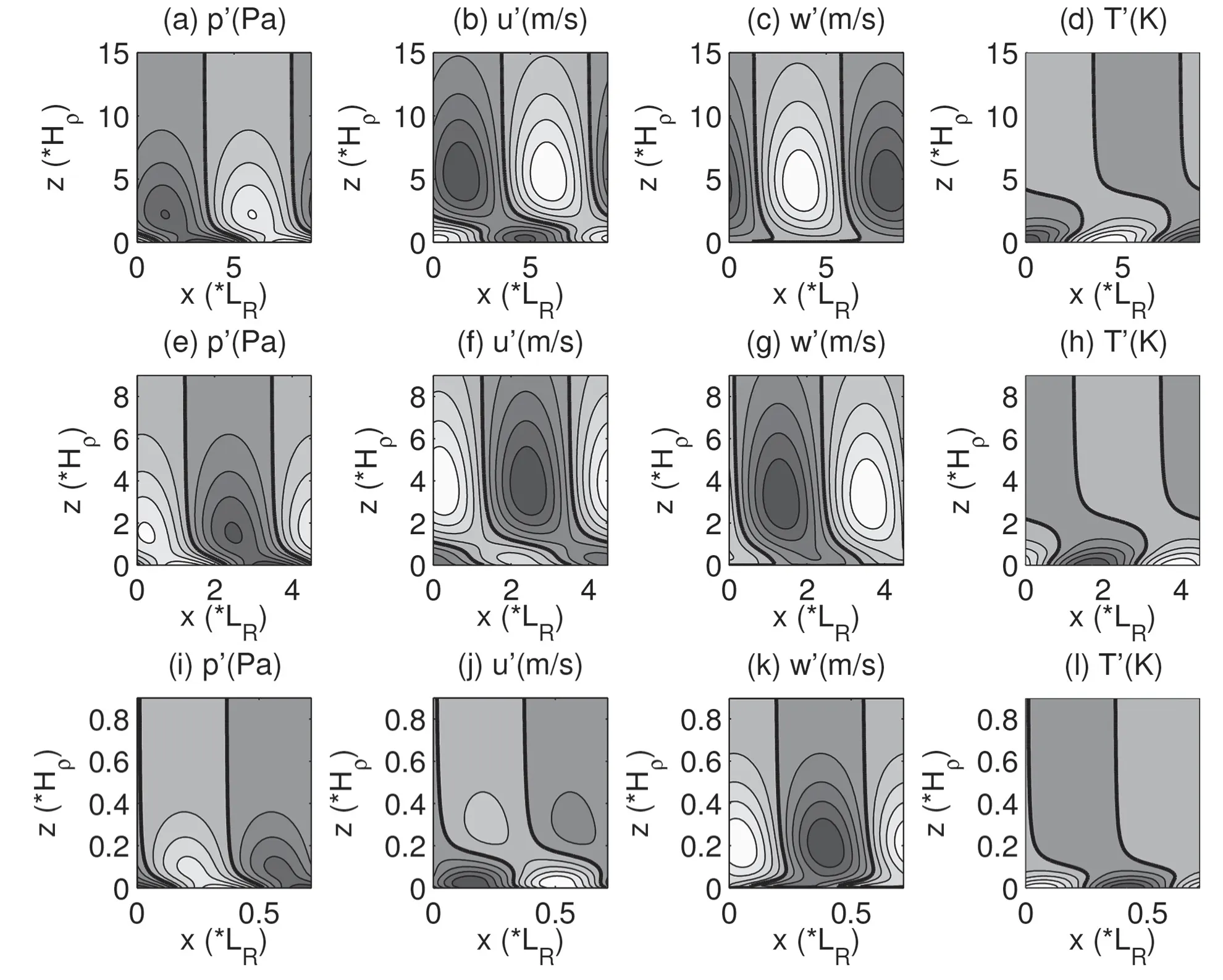
Fig.4.Perturbation f ields at the time instant when the maximal pis taken to be 10 hPa at the surface:(a–d)γ=0.1,(e–h)γ=1,and(i–l)γ=10.Thef ield in each subplot hasbeen normalized by itsmaximum.Thescaleheight Hρ=8800 m,and the Rossby radius L R=1218 km.

4.MS-EVA analysis

4.1.MS-EVA setup

Thedataset obtained is in Cartesian coordinates.The series span four periods,which are divided into 28time steps.In the x-direction the domain covers four wavelengths;it is discretized into 200 grid points.In the y-direction f ive grid points are chosen,with a spacing the same as∆x.In the vertical,300 levelsfrom bottom up are selected.Since what we are concerned with is the interaction between the basic state and theperturbations,thebackground-scalebound j0ischosen to be zero.In Liang and Anderson(2007),it was proven that thismakesaf ield precisely itscorresponding mean f ield.

For thisstudy,threetypical casesarechosen(refer to Fig.4),i.e.,two extreme cases(the deep mode limitγ=0.1 and the shallow mode limitγ=10)and a moderate case(γ=1).The parametersof the corresponding mean f lowsarelisted in Table2.Given thevaluesof theseparameters,themean f ields can begenerated asshown in section 3.1.A reconstruction of the mean state of the Charney model asγ=1 is shown in Fig.5.Finally,themean f ields,together with theperturbation f ields,form theinput of MS-EVA.

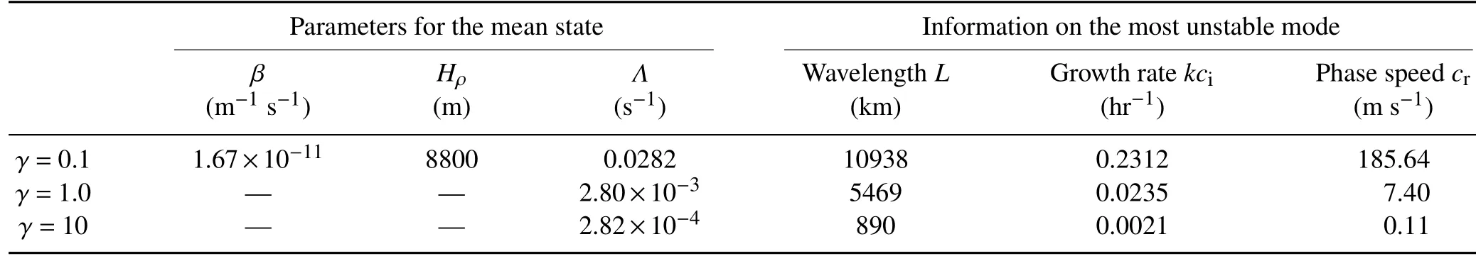
Table 2.Values of the key parameters of the mean states and the corresponding most unstable modes of the three selected cases.

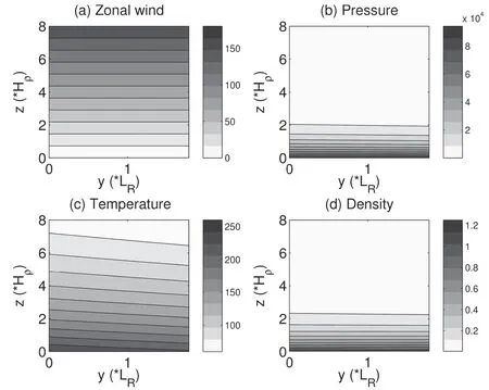
Fig.5.Mean state of Charney’s model asγ=1:(a)zonal velocity(m s−1);(b)pressure(Pa);(c)temperature(K);and(d)density(kg m−3).

4.2.Resultsanalysis:γ=1

4.2.1.Perturbation f ields

With the datasets generated,a two-scale decomposition isperformed for each f ield.To present theperturbation f ields,we need only consider a particular instant.This is because,as a result of linearization,solutions of the Charney model are similar at all times,only with variations of magnitude and phase.Any snapshot of a f ield is typical of the evolution pattern of that f ield throughout the duration.Hereafter,wechoosethetimeinstant,at which themaximal valueof pon the surface is taken to be 10 hPa,to display the energetics.Moreover,asestablished by predecessors(and mentioned before in this study),themost unstable mode corresponds to the y-wavenumber l=0,which implies that the instability structure is y-independent.Therefore,only one x–z section is enough for theanalysis.

The perturbation f ields are expected to be reconstructed precisely on theperturbation-scalewindow;for example,p∼1should be equal to p,T∼1should be T,etc.,and this is indeed true(not shown).The distributions of eddy(i.e.,perturbation)APE(EAPE)and eddy kinetic energy(EKE),def ined by Eqs.(1)and(2)asγ=1,are shown in Fig.6.Obviously,both EAPEand EKEare bottom-trapped.On the EAPEmap(Fig.6a),the trapping is especially strong,with most EAPE generally limited below thesteering level(0.3Hρ).Abovethat height,EAPE still exists,though in very small quantities;in fact,on thezonally averaged EAPEprof ile,above1Hρ,there isadistinctly increasing trend with height(Fig.6b).Thisfeature seems to be odd but very robust(refer to the inset plot in Fig.6b).We shall get back to this point in the following subsection.

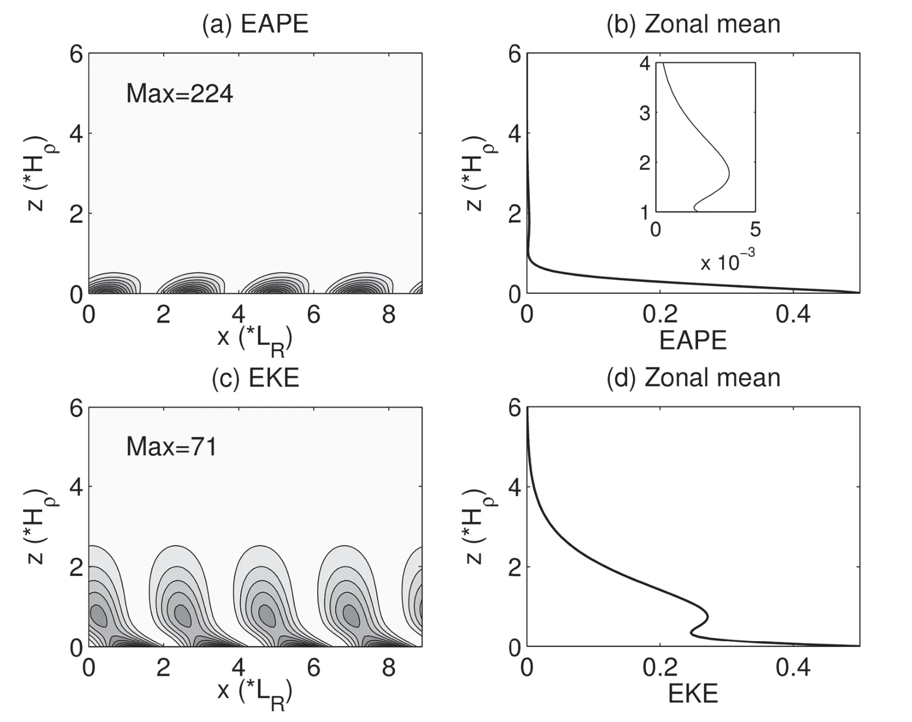
Fig.6.EAPE(m2 s−2)and EKE(m2 s−2):(a)zonal section of EAPE;(b)zonal-mean EAPE;(c)zonal section of EKE;and(d)zonal-mean EKE.

EKE is more colorful in structure(Fig.6c).Apart from thebottom-trapping feature,thedistribution hasan appealing structure.Below 1Hρ,it tilts to the west with height;above that,it becomes almost vertical.Besides,a secondary maximum center occurs at around 1Hρwhere EAPEgets its minimum.This is more obvious in the zonally averaged prof ile(Fig.6d).We discussthis further later in the paper.

4.2.2.Baroclinic and barotropic canonical transfers

Thecanonical transferscorrespond precisely to theinstabilitiesingeophysical f luid f lows.Wehencef irstlook atthese f ields.Shown in Figs.7a and b arethesectional distributions of the baroclinic transfer(BC)and its zonal average,respectively.Generally,itispositivebelow 2Hρ;thatisto say,in the lower layer a baroclinic instability occurs,and theinstability strength increasestoward thebottom.Above2Hρ,BCiseven negative,though weak.In other words,thezonal f low within that layer isbaroclinically stable.

The barotropic canonical transfer(BT)is by comparison two orders of magnitude smaller.What makes it merit particular attention isthat it has acompletely di f f erent structure(Figs.7c and d).Itsvariation in thezonal direction istrapped in the middle layer.The zonal-mean BT takes its maximum at about 0.6Hρ,and vanishesat the top as well asthe bottom.Since it is positive throughout the vertical extent(except for thebottom),barotropic instability isoccurring throughoutthe f luid column,but with an intensif ication in the middle and lower layers(between 0.5Hρand 3Hρ).Note that 1Hρisthe height where BC tends toward zero.This explains why the tilting begins to inf lect back at this height on the maps of uand p(Fig.4),sincethetilting signif iesbaroclinic instability but not barotropic instability.

The distribution of the total canonical transfer(BC plus BT)is quite similar to that for BC,especially in lower layers(below 1.5Hρ),as BT is very small compared to BC(Fig.8a).Their di f f erence occurs in the middle-to-upper layers.Above 1.5Hρ,BT can be many times larger than BC,which is negative(Fig.8b).Together,they give a positive value.This means that the system is unstable,and the instability is mainly baroclinic.Besides,the baroclinic instability is bottom-trapped,agreeing with the traditional conclusion with the Charney model(e.g.,Charney,1947;Kuo,1952;Green,1960;Bretherton,1966;Edmon et al.,1980).However,here,wef ind that theinstability isnot purely baroclinic.BT,though two orders of magnitude smaller,has a distinctly di f f erent structure.In fact,according to itsformula(ΓK)in section 2,the positive BT here is mainly a release of the kinetic energy of the vertical shear.As we will see soon below,it is this barotropic instability that causes the perturbation f ieldsto deviatefromapurebottom-trapped picture.Therefore,strictly speaking,the system is undergoing a mixed instability.

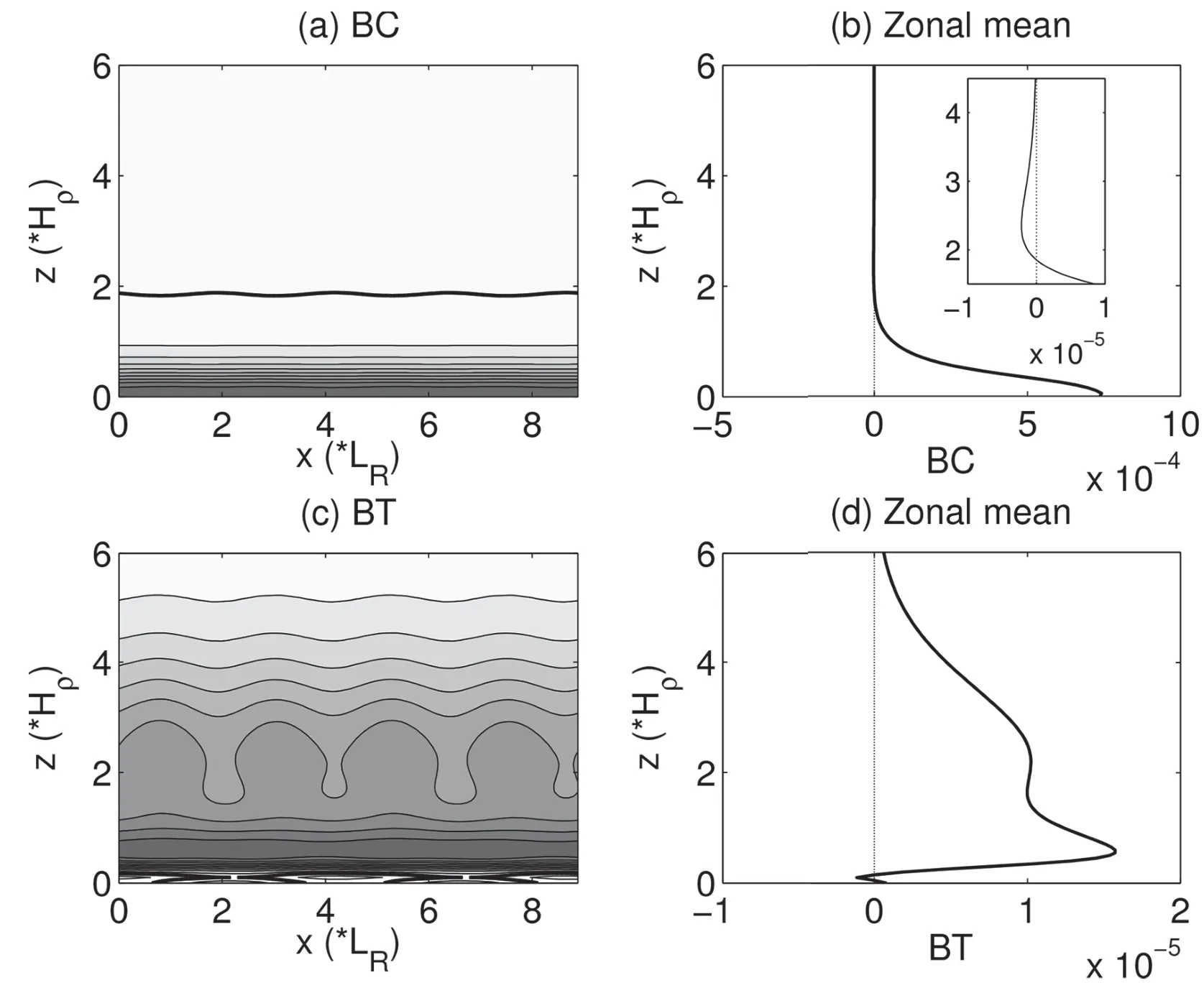
Fig.7.BC(m2 s−3)and BT(m2 s−3):(a)zonal section of BC;(b)zonal-mean BC;(c)zonal section of BT;and(d)zonal-mean BT.

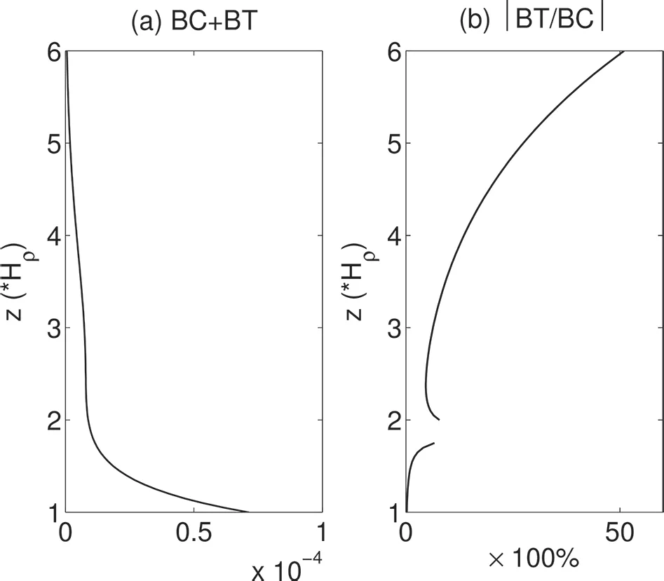
Fig.8.Vertical prof ilesof(a)thetotal energy transfer(BCplus BT),and(b)theratio of BCand BT.Note that the gap around z=2Hρin(b)is left intentionally since BCis almost zero there.

4.2.3.Multiscaleenergy balance

The canonical transfers allow usto reconstruct the instability structures.Onewould expect that they can explain the particular distributions of the perturbation energies.This is,however,not completely true here.Comparing Fig.7 to Fig.6,it is apparent that BC is negative above 2Hρ,while EAPE doesnot vanish there.Instead,a secondary EAPEcenter occursthere.Onewould naturally ask how thesystem gainsits APEwhere thereisno baroclinic instability at all.In thefollowing,this,together with other issues,is addressed through a detailed analysis of the MS-EVA terms.

We f irst look at the perturbation buoyancy conversion(b1).Buoyancy conversion is important in that it mediates between KE and APE and,in fact,is the only connection between KE and APE.It is an important process in the atmosphere and ocean,which also exists in quasi-geostrophic movements.Moreover,therearemany studiesconcerning the buoyancy conversion process in idealized quasi-geostrophic models,such as Green(1960,1970),Gall(1976b),Lapeyre and Klein(2006),Ragone and Badin(2016),etc.Drawn in Figs.9a and b are,respectively,the sectional distribution of b1and its zonal average.A conspicuousfeature is,again,the bottom-trapped negativeconversion,i.e.,theconversionfrom EAPEto EKE,with amaximum(in magnitude)taking place around 0.4Hρhigh.Theconversion,however,reversesitsdirection at the upper levels.That is to say,now it becomes positive,though by comparison the conversion rate is much smaller.Thecritical height where the reversion takes placeis about 2Hρ(refer to the inset plot in Fig.9b).A similar vertical structure of b1can be seen in previous studies,such as Green(1970),Gall(1976b),Branscome(1983),etc.

It should be pointed out that,besides the importance itself as a mechanism for energy to convert,buoyancy conversion has been extensively utilized in the literature for localized baroclinic instability studies(e.g.,Gill,1982).Thisis becauseof itslocalized nature,freeof spatial averagingor integration,plusan intuitiveargumentthat anegativebuoyancy conversion,i.e.,a net conversion of EAPEto EKE,implies a baroclinic instability.While this may seem to be true sometimes,physically it is groundless.If one goes back to the fundamentals,one f inds baroclinic instability and buoyancy conversion are two completely di f f erent concepts.They may correspond well on exceptional occasions,but generally the correspondence may not be seen,as has been evidenced in realistic problems(e.g.,Zhao et al.,2016).In this problem,themaximal conversion(around 0.4Hρ)does not correspond to themaximal baroclinic instability(at thebottom),either.

Next,we look at the multiscale transport processes,i.e.,which are represented by the QQQ terms in the MS-EVA balance.Here,wehaveonly thesetermsontheperturbation window.Plotted in Figs.10aand c arethehorizontal(−)and vertical(−components of the EAPE f lux convergence,respectively,and their corresponding zonal averages(Figs.10b and d).The zonally averaged−∇·is zero throughout the whole depth.This implies that EAPEis transported horizontally withoutitsvertical distribution being changed,whereas another mechanism—namely,the vertical f lux—ismainly to transport EAPEfrom themiddlelayer(between 0.3Hρand 1.2Hρ)to thebottom layer.

On the EKE,thetransport processescould bedueto both theconvergenceof EKEf lux(−∇·QQQ1K)and thepressuref lux(−∇·QQQ1P),either of which,asthat for−∇·QQQ1A,hasahorizontal component and avertical component.Like−∇·QQQ1A,h,the zonal average of−∇·QQQ1K,his zero(Fig.10f).For−∇·QQQ1K,z(Fig.10h),it is positive below 2Hρand negative above.Its maximum and minimum centers occur at 0.3Hρand 3Hρ,respectively.This implies that−∇·QQQ1K,zcontributes to the bottom trapping of EKE.Pressure working rate is quite differently,as shown in Figs.10i-h.Firstly,both−∇·QQQ1P,hand−∇·QQQ1P,ztilt toward the west with height below 2Hρ,above which the phaseline isalmost vertical(Figs.10iand k).Second,the zonal-mean prof ile of−∇·QQQ1P,halmost varnishes(Fig.10j),whereas−∇·QQQ1P,ztakes its minimum and maximum at 0.3Hρand 1.5Hρ,respectively,and beginsto change sign at 1Hρ(Fig.10l).Thevertical extent between 0.4Hρand 1.5Hρcorrespondsto the inf lection region in thezonal-mean distribution of EKE(Fig.6d).

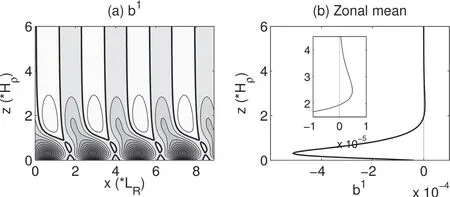
Fig.9.(a)Zonal section of buoyancy conversion(m2 s−3),and(b)the zonal average.

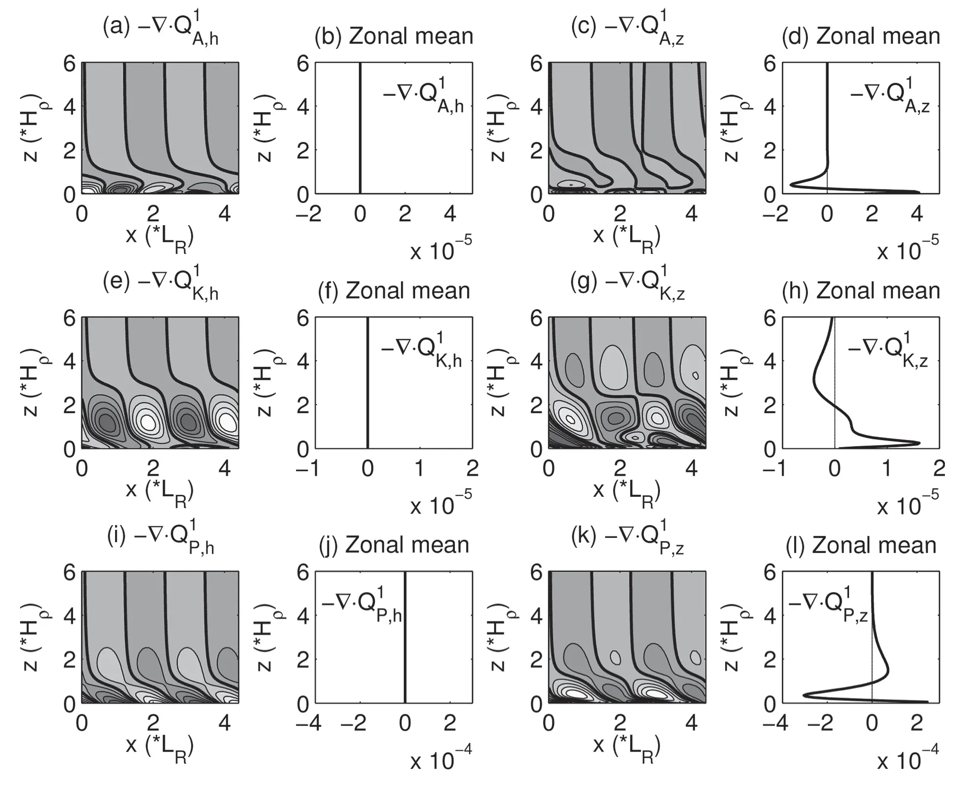
Fig.10.(a–d)Horizontal and vertical EAPE f lux convergences(m2 s−3):(a)zonal section of−∇·QQQ1A,h;(b)zonal-mean−∇·QQQ1

A,h;(c)zonal section of−∇·QQQ1A,z;(d)zonal-mean−∇·QQQ1A,z.(e–h)As in(a–d),but for the EKE f lux convergences(−∇·QQQ1K,hand−∇·QQQ1K,z).(i–l)Asin(a–d),but for pressuref lux convergences(−∇·QQQ1P,hand−∇·QQQ1P,z),respectively.

From the above observations,the energetics scenario is now clear.We summarize it in Fig.11.From the f igure,the system is undergoing a baroclinic instability at the bottom,and most of the APE extracted at a height from the basic temperature f ield essentially remains at that height,causing

Tf ieldsto grow.Tisonly horizontally transported through EAPE f lux without their magnitudes changing;in contrast,EAPE is transported from the middle layer to the bottom through the vertical EAPE f lux to f ill the depletion of EAPE by buoyancy conversion.A part of EAPE is converted to EKE.The conversion takes place from the bottom through 2Hρ,and is maximized at 0.4Hρ.The converted energy at a level,however,doesnotremainatthatlevel;rather,itistransported upward and downward through pressure f lux.Consequently,EKEfrom theconversion isconcentrated toward the bottom by−∇·QQQ1K,z.Besides,theuniquevertical distribution of−∇·QQQ1P,zcausesthezonally averaged EKEprof iletoinf lect between 0.4Hρand 1.5Hρ,and the secondary EKE center at 1Hρ.The scenario here is generally consistent with that described by Gall(1976a).

On theother hand,thesystemalsoundergoesabarotropic instability,though much weaker.In contrast to the bottom trapping of its baroclinic counterpart,it takes place throughout thecomputational domain,intensif ied at middle-to-upper levels.This instability causes the system to extract energy fromthebackground f low tofuel theperturbationf low,which makesthesecond extremecenter in thef ield mapsof u(Fig.4f)and themiddle-level maximum of w(Fig.4g).The EKE,however,doesnot all go to theperturbation f low;asmall part of it isconverted into EAPE.Thiscan beseen from thebuoyancy map(Fig.9b),which becomes positive above 2Hρ.In fact,this is the very reason why there is a small amount of EAPEin theupper domain(Fig.6b),though thereisno baroclinic instability there.

4.3. Results analysis:γ=0.1 andγ=10

4.3.1.Perturbation energy

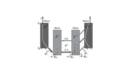
Fig.11.Schematic illustration of theinstability and energeticsscenario in Charney’s model asγ=1.The small arrows in the diagram indicate the directions of various vertical transports(f luxes),with the width and length signifying the transport strength.Refer to the main text for details.

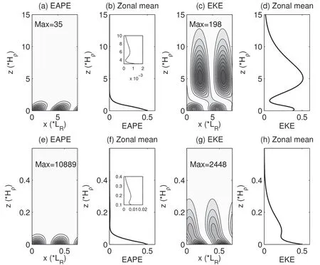
Fig.12.As in Fig.6,but for(a–d)γ=0.1 and(e–h)γ=10.

Figure 12 shows the sectional distributions and vertical prof ilesof thetwo limiting cases.Aswe can see,in the deep mode limit(γ=0.1),EAPE is still bottom-trapped with a secondary maximum center at 6Hρ(Fig.12b),whereas the bottom trapping of EKE becomes moderate and its middlelevel center at 5Hρis much stronger than its bottom counterpart(Fig.12d).In the shallow mode limit(γ=10),the bottom trapping intensif ies.Both maximum centersof EAPE and EKEhappen on thesurface.Besides,thesecondary EKE center weakens greatly(Fig.12h),whereas that of EAPE at 0.2Hρisstrengthened in arelativesense(Fig.12f).

4.3.2.Canonical transfer

Figure 13 shows the vertical prof iles of BC and BT of thetwo limiting cases.It issurprising to f ind that therelative importance of BC and BT varies withγ.In the deep mode limit,BC(Fig.13a)and BT(Fig.13b)have almost the same magnitude,with the latter even stronger than the former.BC isstill bottom-trapped(below 5Hρ),but itsmaximum occurs abovethesurfacerather than on it.BT ispositivethroughout thewholedepthexceptatthebottom.Vertically,therearetwo maximum centers:oneisat 1.5Hρ,and theother at 7Hρ.The upper-level center is much stronger than the lower one.On thecontrary,in theshallow modelimit,BC(Fig.13c)isfour ordersof magnitudelarger than BT(Fig.13d).Therefore,the system canbeviewed aspurely baroclinic.Notethat in either these two limiting cases(γ=0.1 andγ=10)or the moderate case(γ=1),BC is always negative in upper levels(Figs.7b,13a and 13c),indicating that the system is baroclinically stableabove a certain level.

4.3.3.Energy balance

The energetics balance also depends onγ.Figure 14 shows the vertical prof iles of the zonally averaged b1,−∇·QQQ1A,z,−∇·QQQ1K,z,and−∇·QQQ1P,z.Wecan seethat thestructures are generally similar to those ofγ=1,but with a big difference in magnitude.For the deep mode,b1,−∇·QQQ1K,zandhave the same magnitude,two orders larger than(Fig.14b).b1is negative below 7Hρand positive above(Fig.14a).−∇·QQQ1K,zisvery strong and it hastwo maximumcenterscorrespondingtothatof EKE(Fig.14c).Therefore,together with BC(Fig.13a)and BT(Fig.13b),the energy f low isthat theperturbation obtains APEfrom themean f low viabaroclinic instability atlow levels.Mostof the EAPE is then converted to EKE through b1and the remaining part istransported downward by EAPEf lux.Meanwhile,thef low isalso undergoing astrong barotropic instability.Thekinetic energy transfer from themean f low to theperturbation mainly happens at upper levels.Then,EKE is transported via EKE f lux and pressuref lux to thelower levels.Therefore,thelowlevel EKEcenter benef itsfrom both BCand BT,whereasthe upper-level EKE center arises mainly from BT.In the upper layer,asmall part of EKEisconverted to EAPE,maintaining thesecondary upper-level center in T.

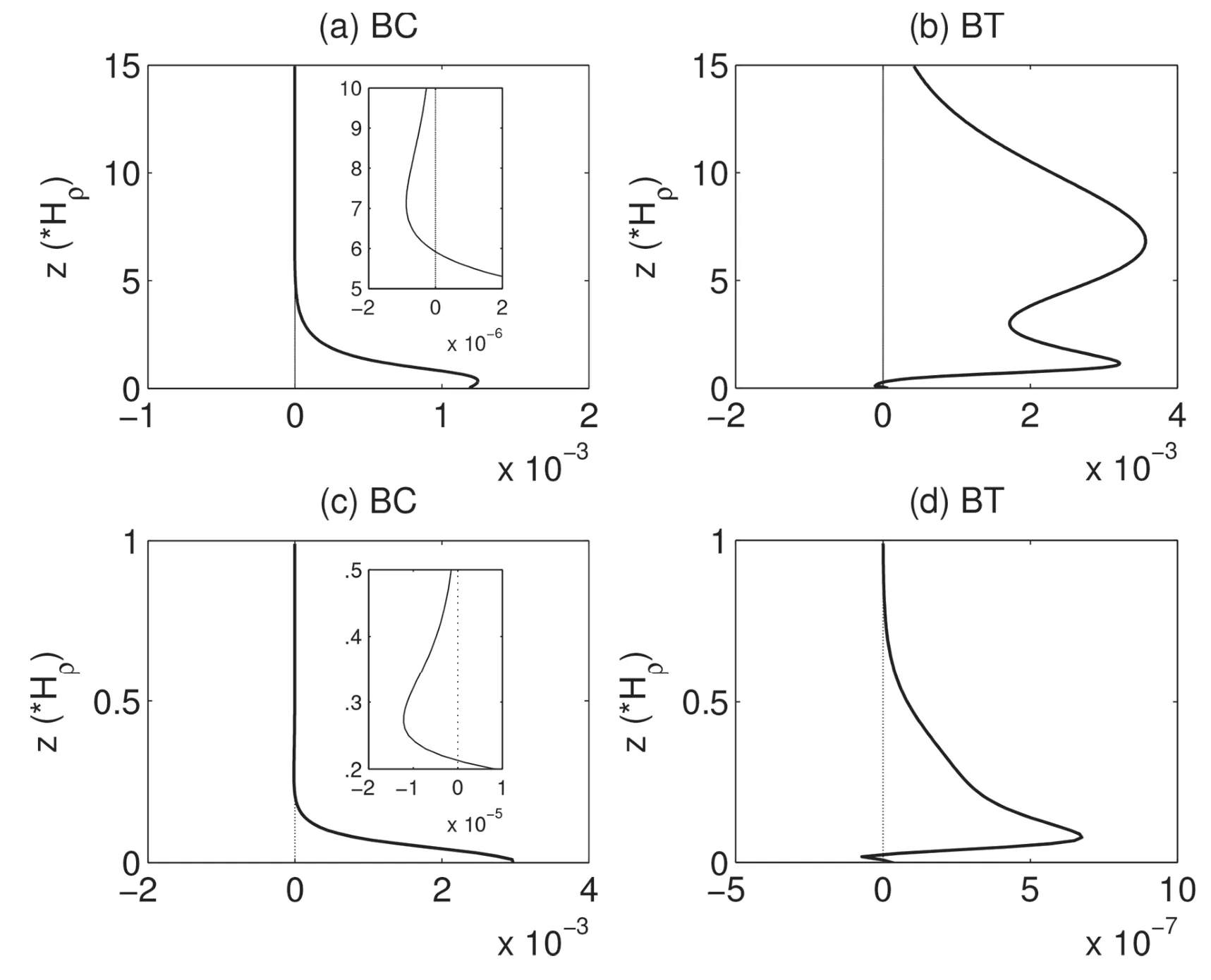
Fig.13.Vertical prof iles of zonal-mean(a,c)BCand(b,d)BT:(a,b)γ=0.1;(c,d)γ=10.

For the shallow mode,the perturbation energy is mainly balanced by threeprocesses,i.e.,BC(Fig.13c),b(Fig.14e),and−(Fig.14h),since BT(Fig.13d),−∇·QQQ1A,z(Fig.14f),andz(Fig.14g)areseveral ordersof magnitude smaller.b1is negative and positive below and above 0.2Hρ,respectively(Fig.14e).−∇·QQQ1P,zis positive at the surface,negative in the lower layer,and positiveat upper levels(Fig.14h).Theenergy balancethereforebecomesstraightforward.Theperturbation f irst obtains EAPEthrough BCin lower levels;then,part of it is converted to EKE;meanwhile,pressure f lux transports EKE to the bottom and upper levels,which results in the secondary center on uand p;at upper levels,EKE is converted back to EAPE,resulting in the secondary center in T.

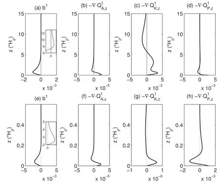
Fig.14.Asin Fig.13,but for theconversion and transport terms:(a–d)γ=0.1;(e–h)γ=10.

4.4. Correspondencein the real atmosphere

As presented above,we have found that the Charney model,which has been considered as a purely baroclinic model,actually also experiences barotropic instability processes.That is to say,apart from the energy from baroclinic canonical transfer,barotropic canonical transfer is also an important source of energy for the most unstable Charney mode.This phenomenon has actually been observed in the real atmosphere.Thewavesover East Asia,which havebeen claimed to be of baroclinic origin,reveal similar behavior.Our recent study(Zhao et al.,2018)showed that thesewaves have two sources in East Asia:a northern one,which is located on the lee side of the Mongolian Plateau at middle and high latitudes;and a southern one,which generally coincides with the East Asian subtropical jet.MS-EVA diagnoses show that the waves in the southern branch experience strong baroclinic instability in the middle and lower layers,and strong barotropic instability in the upper layer;whereas,in the northern branch,the waves derive mainly from baroclinic instability[cf.Figs.6 and 8 in Zhao et al.(2018)].It isworth noting that thesouthern branch wavesarelocated in the center of the jet stream,where the vertical shear is large,whereasin thenorth thevertical shear issmall.Thesescenarioscorrespond qualitatively to the casesofγ=1 andγ=10,respectively,in thisstudy.

It should benoted that,although thesecond maximum of theeddy energy in theupper levelsin the Charney model can correspond to theobserved second peak of eddy activity near the tropopause(e.g.,Kao and Taylor,1964;Lorenz,1967),they actually comefrom di f f erent mechanisms.Asdiscussed above,the upper-level energy center in the Charney model is largely attributed to barotropic instability,whereas that observed near the tropopause is mainly due to buoyancy conversion and vertical transport of energy(e.g.,Simons,1972;Gall,1976a;Simmons and Hoskins,1978).Moreover,in the real extratropics,kinetic energy is mainly transferred from eddy to mean f low(e.g.,Chang and Orlanski,1993),which is opposite to that in the Charney model;and this process is mainly caused by thehorizontal shear of thebackground f low(e.g.,Deng and Mak,2006;Zhao et al.,2018),whereas the Charney model does not at all have horizontal shear in the basic wind.

5.Conclusions

The Charney model is reinvestigated using the MS-EVA method developed by Liang and Robinson(2005)[see Liang(2016)for the updated version],which is based on a novel functional analysis tool—namely,the MWT(Liang and Anderson,2007).For the f irst time,we are able to obtain a relatively complete instability structure,though this model as a prototype of baroclinic instability has been extensively studied before.Di f f erent from the traditional belief,the Charney model actually undergoes a mixed instability;that is to say,the instability is both baroclinic and barotropic,which are represented respectively by baroclinic canonical transfer(BC)and barotropic canonical transfer(BT)in the MS-EVA.Theresulting BChasavertical distribution agreeing with the traditional results,i.e.,it isbottom-trapped,almost vanishing at the middle and upper levels.However,BC alone cannot explain why there exist temperature oscillations at the upper levels,and why thereisasecond extreme on theperturbation f low and pressuref ields.Our study showsthatabarotropic instability,though much weaker for most of the cases,actually existsthroughout the f luid column.In the bottom region,it is overwhelmed by the baroclinic instability,but above that region where BCissmall,itse f f ectbecomessignif icant.So,the instability isactually amixed one.Besides,itisfound thatthe relativeimportanceof baroclinic instability and barotropic instability varies with the Charney–Green numberγ,the ratio of atmosphere scale height Hρ,and the perturbation vertical scale.In the shallow mode limit(γ1),barotropic instability is so weak that the system can be viewed as purely baroclinic.But,in the deep mode limit(γ1),barotropic instability isstrong;in fact,it can beeven stronger than baroclinic instability.

Accordingly,the energy balance and the maintenance of theupper-level centersin p,u,and Tin the Charney model also depend onγ.Whenγ1,BCisseveral ordersof magnitude larger than BT.Therefore,the system can be viewed as purely baroclinic,and the energy source is BC only.The scenario of the energetics processes can be summarized as follows:First,the system receives EAPE through baroclinic instability at the bottom.Then,most of the extracted APE goesto theperturbation temperatureand causesitto grow,but asmall part isconverted into EKE,and theconverted EKEis brought downward and upward through pressuref lux,resulting in the bottom-trapped feature and the secondary centers in uand p.In theupper levels,apart of the EKEtransported by pressure f lux is converted to EAPE,leading to the formation of the secondary center in T.

In contrast,for smallγ,BC and BT are of the same order of magnitude.The energetics scenario is as follows:At the bottom,the system is undergoing a baroclinic instability.Most of the extracted APEgoes to the perturbation temperature and causes it to grow,but a small part is converted into EKE,and the converted EKE is brought downward through pressure f lux and EKE f lux,making the perturbation f low f ields become trapped at the bottom too.In the meantime,the system is also undergoing a barotropic instability,which becomesdominantatmiddle-to-upper levels,wherethebaroclinic instability stops functioning,and where the tilting on the maps of uand pbecomes rectif ied.This explains why there is a second extreme center on the perturbation f low maps,and why EKE has an inf lection on its vertical prof ile.Besides,a part of the EKE through the barotropic instability is converted to EAPE,providing the energy source for theobserved oscillationsof temperatureat theupper heights,which,though identif ied long before,have been generally overlooked.

Acknowledgements.The suggestions of the two anonymous reviewers are appreciated.Yuan-Bing ZHAO thanks Yang YANG,Yi-Neng RONG,and Brandon J.BETHEL for their generous help.This research was supported by the National Science Foundation of China(Grant Nos.41276032 and 41705024),the National Program on Global Change and Air–Sea Interaction(Grant No.GASIIPOVAI-06),the Jiangsu Provincial Government through the 2015 Jiangsu Program of Entrepreneurship and Innovation Group and the Jiangsu Chair Professorship,and Shandong Meteorological Bureau(Contract No.QXPG20174023).