Climate and Vegetation Driversof Terrestrial Carbon Fluxes:A Global Data Synthesis

Shutao CHEN,Jianwen ZOU,Zhenghua HU,and Yanyu LU

1Jiangsu Key Laboratory of Agricultural Meteorology,Nanjing University of Information Scienceand Technology,Nanjing 210044,China

2College of Resources and Environmental Sciences,Nanjing Agricultural University,Nanjing 210095,China

3School of Applied Meteorology,Nanjing University of Information Science and Technology,Nanjing 210044,China

4Climate Center,Anhui Weather Bureau,Hefei230031,China

ABSTRACT The terrestrial carbon(C)cycle plays an important role in global climate change,but the vegetation and environmental driversof Cf luxesarepoorly understood.Weestablished aglobal dataset with 1194 availabledataacrosssite-yearsincluding grossprimary productivity(GPP),ecosystem respiration(ER),net ecosystem productivity(NEP),and relevant environmental factors to investigate the variability in GPP,ER and NEP,as well as their covariability with climate and vegetation drivers.The results indicated that both GPPand ER increased exponentially with the increase in mean annual temperature(MAT)for all biomes.Besides MAT,annual precipitation(AP)had a strong correlation with GPP(or ER)for non-wetland biomes.Maximumleaf areaindex(LAI)wasan important factor determining Cf luxesfor all biomes.Thevariationsin both GPPand ERwere also associated with variationsin vegetation characteristics.Themodel including MAT,APand LAIexplained 53%of the annual GPPvariations and 48%of the annual ER variations across all biomes.The model based on MAT and LAI explained 91%of theannual GPPvariationsand 92.9%of theannual ERvariationsfor the wetland sites.Thee f f ectsof LAI on GPP,ER or NEPhighlighted that canopy-level measurement is critical for accurately estimating ecosystem–atmosphere exchangeof carbon dioxide.Thepresentstudy suggestsasignif icanceof thecombined e f f ectsof climateand vegetation(e.g.,LAI)driverson Cf luxes and shows that climateand LAImight inf luence Cf lux components di f f erently in di f f erent climate regions.

Key words:net ecosystem productivity,gross primary productivity,ecosystem respiration,controlling factors,vegetation,model

1. Introduction

Theglobally averaged air temperaturehasshown awarming trend sincethe industrial revolution(IPCC,2013).Given that theterrestrial carbon(C)cycleplaysan important rolein global warming,it iscritical to understand thekey controlsof the C metabolism of terrestrial ecosystems(Canadell et al.,2007).Over the past several decades,terrestrial ecosystems have generally been regarded as C sinks(Houghton,2007),and the magnitude of terrestrial ecosystems in sequestering atmospheric carbon dioxide(CO2)is of interest in mitigating climate changes because this terrestrial sink counters the anthropogenic increase in atmospheric CO2levels.Friedlingstein et al.(2006)found that C–climate feedback was positive.Atmospheric CO2enters terrestrial ecosystems through photosynthesis,and terrestrial C is released back to the atmospherethrough a variety of processes,collectively referred to asrespiration(Trumbore,2006).

Generally,the components of C f lux include gross primary productivity(GPP),ecosystem respiration(ER),and net ecosystem production(NEP)(thedi f f erencebetween GPP and ER)(Reichstein et al.,2005).Eddy covariance is a method used in meteorology and other applications(e.g.,micrometeorology and hydrology)to determineratesof gaseous exchange(Baldocchi,2008).With the establishment of eddy covariance sites and relevant meteorological and biological measurements(Baldocchiet al.,2001;Valentiniet al.,2000),a large body of data is available on the terrestrial ecosystem exchange of mass at stand level(Law et al.,2001;Wang et al.,2017).Measurements of GPP,ER and NEPare needed in order to determine the source–sink status of a specif ic ecosystem and to analyze how CO2exchange varies with the temporal variation in environmental conditions(Flanagan et al.,2002;Schmitt et al.,2010).Site-level observationshavegreatly advanced our understanding of patterns and environmental controls of terrestrial ecosystem C f luxes(Xu et al.,2014).

Thetemporal and spatial dynamics of GPP,ERand NEP are di f fi cult to model or predict.Modeling e f f orts linking with observations at yearly scales are critical to progress in the f ield of terrestrial C f luxes.Analysis of global C f lux data based on eddy covariance measurements makes it possible to identify ecosystem-scale CO2f lux patterns that are not determined well in individual studies(Baldocchi,2003;Baldocchiet al.,2015).The C f lux measurements from individual studies have been synthesized to evaluate patterns of ecosystem C f luxes at regional(Valentiniet al.,2000;Law et al.,2002;Kato and Tang,2008;Chen et al.,2013;Yu et al.,2013;Xiao et al.,2013;Chen et al.,2019)and global scales(e.g.,Luyssaert et al.,2007;Baldocchi,2008;Yuan et al.,2009;Beer et al.,2010;Mahecha et al.,2010;Xu et al.,2014;Shao et al.,2015;Jung et al.,2017;Zhang et al.,2018).Although several studies have analyzed thespatial patternsof global Cf luxes(Luyssaert et al.,2007;Migliavaccaet al.,2011;Chen et al.,2015;Jung et al.,2017;Zhang et al.,2018),their datasets did not include all of the Cf lux data pointsworldwide and relevant vegetation characteristics[e.g.,litterfall(LF),treeage(TA),diameter at breast height(DBH),treeheight(TH),and basal area(BA)].Despite hundredsof f lux measurement sites,theavailability of Cf lux data remains an important challenge for global synthesis.A large number of data points have been published in various literatures or are available publicly in the global FLUXNET(http://f luxnet.f luxdata.org/).Establishing such a dataset and synthesizing by using the data fusion technique can help in understanding the mechanisms of the C cycle and assessing the magnitude of the Cbudget(Wang et al.,2009).

It islikely that Cf luxesvary across di f f erent biometypes(e.g.,non-wetland versus wetland),climate zones,and vegetation conditions.The inf luence of climate on C f luxes has been examined by several studies(e.g.,Kato and Tang,2008;Beer et al.,2010;Mahecha et al.,2010;Xiao et al.,2013;Chen et al.,2015).For instance,Kato and Tang(2008)indicated that CO2f luxes—particularly annual NEP—are determined mainly by mean annual temperature(MAT)and annual precipitation(AP).A global synthesisshowed that GPP and ER are also related to MAT and AP(Chen et al.,2015).Our knowledgeof ecosystem Ccycling and itsvariability has been improved by investigating the global relationships between observed climate and site-level biosphere–atmosphere f luxes(Stoy et al.,2009).We have understood broadly how temperatureand precipitation a f f ectdi f f erent Ccycleprocesses.Whatwedohave,however,isaquantitativeunderstanding of theindividual e f f ectsof temperature and precipitation and their comprehensivee f f ects.Furthermore,thevegetation and environmental drivers of C f luxes are poorly understood and need to be further addressed.Particularly lacking,to the best of our knowledge,is compiled data focusing on synchronous measurements of NEP and vegetation characteristics and a comprehensiveanalysisof such data.Whether thedependency of C f luxes on climate di f f ers with biome type,vegetation characteristics,or other factorsisnotwell quantif ied.A better understanding of Cf lux dynamicswill comefrom elucidating theintegrated e f f ectsof climateand vegetation constraintson GPP,ERand NEP.Many moredataon Ccycling and vegetation characteristics in various biomes[e.g.,forest,grassland(GL),wetland]make it possible to investigate the vegetation driversof terrestrial Cf luxes.In addition,the Ccycle in wetlands is di f f erent from that in non-wetlands because of its special ecohydrology.The water layer in wetlands reduces soil CO2emissions,resulting in di f f erent C cycle patterns between wetlands and non-wetlands(Bridgham et al.,2006).Some studies that have synthesized f lux observations from wetlands at regional scales typically used observations from afew sites(Turetsky et al.,2014;Petrescu et al.,2015).A recent article by Lu et al.(2017)reported that ecosystem CO2f luxes of both inland and coastal wetlands are mainly regulated by MAT and AP,and the combined e f f ects of MAT and APcan explain 71%,54%and 57%of the variationsin GPP,ERand NEP,respectively.However,thecombined e f f ectsof MAT,AP,and vegetation characteristics[e.g.,leaf areaindex(LAI)]on C f luxes have not been well explained,although many f lux and vegetation measurements in wetlands worldwide have been well documented(e.g.,Hirano et al.,2007;Hao et al.,2011;Beringer et al.,2013;Knox et al.,2015).The key questions that need to be addressed are whether the main driversof Cf luxesin wetlands are di f f erent from those in non-wetlands,and how to model C f luxes in wetlands using climate and vegetation characteristics.

In thepresentwork,weassembled acomprehensiveglobal dataset for terrestrial ecosystems that includes C f luxes(i.e.,GPP,ER and NEP),biome categories,climate factors(temperature and precipitation),and vegetation traits(e.g.,LAI).Although previous hypotheses have proposed that climate and vegetation characteristics may individually inf luence GPP,ER and NEP,the combined modeling of C f luxes on the basis of large-sample data on in-situ simultaneous measurements of climate and vegetation characteristics at the global scale remains lacking.Therefore,our present publicly available dataset is dedicated to re-examining previously hypothesized global relationships and developing new models.The objectives of the study were to:(1)present the dataset’sstructureand explain theglobal patternsof GPP,ER and NEP;(2)identify climate and vegetation drivers of these three f luxes for di f f erent biomes[e.g.,forest,GL,cropland(CL),and wetland];(3)determine the relative contributions of di f f erent drivers to the interannual and inter-site variabilitiesof thesef luxes;and(3)establish modelsthatf itthespatial and temporal variations in C f luxes in di f f erent biomes(wetland,forest,GL,and CL).

2.Materialsand methods

2.1. The dataset

We compiled a dataset of 327 references from 296 sites that were useful for the synthesis analysis[Table S1 in electronic supplementary material A(ESM A)].All of the referencescompiled in thisstudy werepublished inpeer-reviewed journals and covered C f lux data from all continents except Antarctica.The oldest measurement year was 1991.The literature survey was intended to be as inclusive as possible up to 2016.Published studies that report annual NEP,GPP and ERwerecompiled using bibliographic databasesincluding ISIWeb of Science and Chinese Journal Net.The GPP,ER and NEP data compiled in this study were not directly downloaded from FLUXNET,because some of the eddy covariance data from FLUXNET have not been corrected.Instead,the C f luxes that appeared in the literature were used,but only where an appropriate correction method for theraw eddy covariance data was applied.We performed the data collection carefully to ensure the Cf luxes(e.g.,GPP,ERand NEP)and relevant environmental factors in the reviewed literature were used and that no part of them were removed.Studies were included if they met the following criteria:(1)they comprised annual NEPmeasurements only,i.e.,studies of seasonal NEP measured during the growing season were not used;(2)the NEPf ield measurementswere unmanipulated;and(3)f looded rice paddies,fenland,peatland,swamps,bogs,and marshes were considered as wetlands.Rice paddieswere considered together with natural wetlands because the seasonal NEP patterns for f looded rice paddies are signif icantly di f f erent from upland f ields,and land-use change from paddy ricecultivation to upland crop cultivation causes signif icant lossesof C(Nishimuraet al.,2008).

Measurement sites were distributed from 35◦39′S to 79◦56′N latitude and from 157◦25′Wto 172◦45′Elongitude,with most sites situated in the Northern Hemisphere(ESM A,Table S1).A total of 1194 measurements of annual NEPwerecollected from 296 sites,and most included annual GPPand ERmeasurement data.There are870 datapoints for annual GPP and ER.The amount of site-year measurements included in the present dataset is more than that in previous studies(Luyssaert et al.,2007;Migliavacca et al.,2011;Chen et al.,2015).For example,the information on C f luxes,climate data and ecosystem properties(e.g.,TA,TH and LAI)in the study of Luyssaert et al.(2007)was only available for forest ecosystems.Our dataset includes six ecosystem types[CL,forest,GL,shrubland(SL),tundra(TD),and wetland].In our dataset,most sites used the u*correction method to avoid underestimating the nighttime C e f fl uxes(Lloyd and Taylor,1994;Massman and Lee,2002).Other methods,which was applied at relatively fewer sites,were used if the u*threshold was di f fi cult to determine(e.g.,Saitoh et al.,2005;Kato and Tang,2008).We used the reported NEE values with the correction method that best considered thespecif ic circumstancesat each site.

For each study,whenever possible,we also noted the location(i.e.,site name and country),latitude and longitude,measurement period,climate conditions,elevation,maximum C f luxes,soil and heterotrophic respiration(SR and HR),net primary productivity(NPP)and aboveground NPP(ANPP),vegetation characteristics,and soil properties(ESM A,Table S1).Variable categories such as climate conditions and vegetation characteristics are listed in Table 1.Vegetation characteristicsincluded LF,f ineroot biomass(FR),NPP,ANPP,growing season length(GSL),TA,plant density of tree(PD),DBH,TH,BA,and maximum LAI.Soil propertiesincluded soil organic Cstorage(SOC),soil total nitrogenstorage(STN),the ratio of C to N (C/N),pH,clay content(CLA),sand content(SAN),and bulk density (BD).Where MAT and AP were not available in the literature,they were derived from the Center for Climatic Research at the University of Delaware(http://climate.geog.udel.edu/∼climate/html pages/archive.html).Theclimatedatawerematched to thecoordinatesof the NEP study sites using a nearest-neighbor method.The maximum LAI(an important variable)data were compiled based only on studiesthat carried out manual measurements,rather than remote sensing,in order to avoid discrepancies between di f f erent datasets.Other potential variables(e.g.,normalized di f f erence vegetation index and greenness)were not compiled,as they are di f fi cult to measure in-situ when C f luxes aremeasured ataspecif ic site.Thedatawerecategorized into 10 biomes:broadleaf and needleleaf mixed forest(BNMF),CL,deciduous broadleaf forest(DBF),deciduous needleleaf forest(DNF),evergreen broadleaf forest(EBF),evergreen needleleaf forest(ENF),GL,SL,tundra(TD),wetland[including forested wetland(FWL)and non-woody wetland(NWWL)](Fig.1).The FWL included mangrovesand swamps,while the NWWL included marshland,mires,rice paddies,etc.Thereason these10 biometypeswereused wasbased on the consideration that leaf traits(i.e.,broadleaf and needleleaf)may have a considerable inf luence on photosynthesis and respiration.

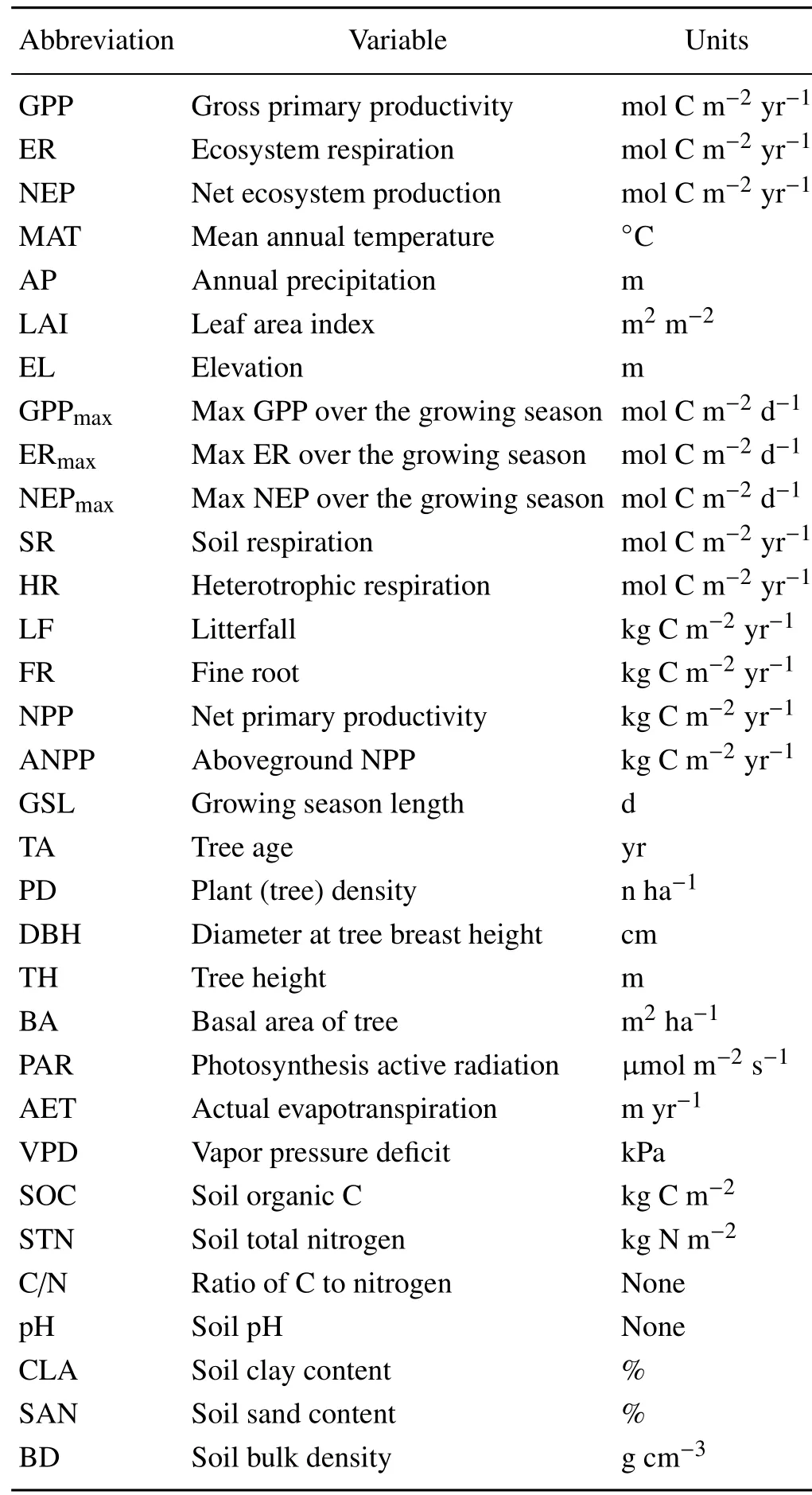
Table1.Variable categories included in the dataset.

2.2. Data analysisand ecosystem modeling

Weexamined thedistribution of annual Cf luxes(i.e.,GPP,ERand NEP)within and acrossbiometypesusingtheboxand-whisker plot.The box-and-whisker plot summarizes a data sample through f ive statistical measures:the minimum,lower quartile,median,upper quartile,and maximum.The mean values of each C f lux were also computed for each biometype.

To clarify the issue as to how MAT and AP inf luenced the C f lux component processes di f f erently,for the growing season length(GSL)and the maximum GPP,ER and NEP,we grouped the global land ecosystems into 12 land climate classes.The scale for AP was divided into less than 0.4 m,0.4–0.8 m,0.8–1.5 m,and greater than 1.5 m,while that for MATwaslessthan10◦C,10◦C–20◦C,and greater than20◦C.The APof 0.4 m,0.8 m and 1.5 m represents the thresholds between semiarid and semihumid zones,between semihumid and humid zones,and between humid and rainy zones,respectively.The10◦Cand 20◦Cpartsof thescalerepresentthe temperature for active growth and vigorous growth of plants,respectively.The GPP,ERand NEPvaluesweregrouped into12 land climateclasses.Thedistribution of annual Cf luxes(i.e.,GPP,ERand NEP)in each climateclasswasdetermined using thebox-and-whisker plot.Moreover,the GSL acrossdi f f erent measurement sites and years could be explained as the MAT-related and AP-related functions,as the GSL was positively correlated with temperature in most climate zones and was closer to the seasonal precipitation pattern in tropical and subtropical regions(Liu et al.,2010;Ngeticha et al.,2014).

To identify the key factors controlling C f luxes,we conducted univariate regression analyses.In the univariate regression analyses,we examined the regulatory mechanisms of C f luxes by climate factors(MAT and AP),vegetation characteristics(e.g.,LAI),and soil properties(e.g.,SOC).The univariate regression analyses were used based on the following considerations.First,only potential factors inf luencing C f luxes with substantial determination coe f fi cients(R2)and very low P values(P<0.001)in the univariate regression analyses can be considered as the variables in the following multivariate models.Second,the distribution patterns of C f luxes and potential drivers can be directly determined in the regression plots,which are necessary in choosing an appropriate mathematical expression in multivariate models.Third,MAT,AP and LAI have been commonly considered as independent predictive factors of C f luxes in previousunivariateregression studies(Luyssaert et al.,2007;Lu et al.,2017;Hursh et al.,2017).Eventually,APonly explained∼10%(R2=0.108)of variationsin LAIwith acorrelation coe f fi cient(r)of 0.328(ESM A,Table S1),whilemost of the variations in LAI(∼90%)could not be explained by APand may contribute to the variations in C f luxes.No signif icant correlation between MAT and LAIwas found on the basisof availabledata(ESM A,Table S1).

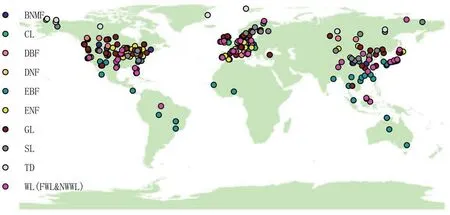
Fig.1.The Cf lux sites compiled in this study.

Several aspects were considered in choosing the key drivers for the C f lux models.First,the models for nonwetlands and wetlands might include di f f erent drivers.Second,both MAT and APwere considered as potential drivers in the model,as they have been found in previous investigations to be important controls of the variability in GPP and ER(Kato and Tang,2008;Chen et al.,2013;Reichstein et al.,2013;Yu et al.,2013;Xiao et al.,2013).Third,only the potential vegetation and soil variables with enough data points and high signif icance can be included in the Cf lux models.When the mainly responsibledrivers(climateand other sitevariables)weredetermined,they wereall included in themodel.

Before establishing the model,the relative contribution of each potential factor to each C f lux was evaluated using the standardized coe f fi cient in stepwise linear regression.To explain the dependence of annual Cf luxeson MAT,AP,and one specif ic environmental control(Xi),we established the following model:

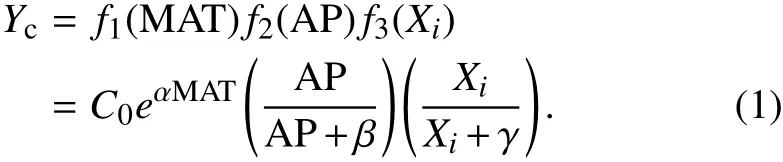
Thismodel considersthe interaction e f f ects among the three variables of MAT,APand LAI,whereas linear models cannot account for the interactions among variables.An exponential model has been commonly used to explain the relationship between C f luxes(GPP,ER and NEP)and temperature(Migliavaccaet al.,2011;Ballantyneet al.,2017).A Michaelis–Menten function suggests declining positive e f f ects of increasing precipitation or another environmental control(Xi)on C f luxes,which has been associated with the water and substrate supply on C assimilation and emission(Migliavaccaet al.,2011;Exbrayat et al.,2013;Ballantyneet al.,2017).This model started from a widely used climate-driven model proposed by Raich et al.(2002)and further modif ied by Reichstein et al.(2003)in the form of a climate-and-LAI-driven model.In the equation,Ycdenotes a specif ic C f lux item(e.g.,GPP);C0is the Ycat 0◦C without precipitation and Xi(one specif ic environmental control)limitations;α(◦C−1)determines the increasing rate of Ycwith the increase of MAT;andβ(m)andγrepresent the half-saturation constants of the Michaelis–Menten function determining the relationship between Ycand precipitation or Xi,respectively.The relationship between precipitation(or Xi)and observed Yccan be approximated using a Michaelis–Menten function,with increasing rates of precipitation(or Xi)having lesser impacts on f luxes.The model’s parameters(C0,α,βandγ)were estimated using aleast sum of residual squares method.The modeling errors were determined by performing abootstrappingprocedureusing resampling from theoriginal dataset to create100 di f f erent datasets(Cameron et al.,2008;Keenan et al.,2013).The GPP,ER and NEPwithin each of the 12 climate classesweremodeled by the climate(MAT and AP)and vegetation variable(LAI)within each climateclass.The model structurewasthesame asin Eq.(1).

Six statistical measures,includingtheadjusted coe f fi cient of determination(R2),probability of obtaining a test statistic(P),root-mean-squareerror(RMSE),model e f fi ciency(ME),mean absolute error(MAE)(Janssen and Heuberger,1995),and Akaikeinformation criterion(AIC)(Akaike,1974),were used to evaluate the performance of the established models.The RMSE,ME,MAE and AIC were computed by the following equations:

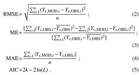
In above equations,Yc,MODand Yc,OBSare the modeled and observed valuesof Cf luxes,respectively;denotes the mean of Yc,OBS,i;n is the number of samples;k def ines the number of parameters in the statistical model;and L is the maximized value of the likelihood function for the estimated model.

All statistical analyseswereperformed with SPSS19.0 for Windows.All levelsof signif icancereported are P<0.05 unlessotherwisenoted.

3.Results

3.1.Variability in GPP,ERand NEPacross biomes

The magnitude of annual C f luxes varied across biomes(Figs.2a–c).Annual GPP and ER of terrestrial ecosystems ranged from3.417to 305.500 mol Cm−2yr−1and from 2.833 to 325.583 mol C m−2yr−1,respectively.On average,EBF had thehighest annual GPPand ER,while TD had thelowest annual GPPand ER.The highest annual GPPand ER were from Simpang Pertang(Malaysia)and Palangka Raya(Indonesia),respectively,while the lowest annual GPPand ER were from Inner Mongolia(China)and Daring Lake(Canada),respectively.Therangeof annual GPPand ERwasgreatest for wetlands,as they included peatland in the tropical zone and fenland in the frigid zone(ESMA,Table S1).For each biome,the mean annual GPPwas slightly higher than the mean annual ER.Annual NEPvaried from−113.333 to 116.667 mol C m−2yr−1(Fig.2c).Compared with GPPand ER,annual NEPshowed lower varianceacrossbiomes.Mean annual NEP was 20.417,17.167,22.417,19.917,25.833,18.750,8.083,4.833,2.833,12.538 and 7.065 mol C m−2yr−1for the BNMF,CL,BDF,DNF,EBF,ENF,GL,SL,TD,FWL and NWWL biomes,respectively.Among the biomes,the highest and lowest mean annual NEPwasfor EBFand TD,respectively.Morethan 80%NEPvaluesweregreater than zero,indicating most examined ecosystems across sites and yearswere Csinks.Thepresent GPPand ERdataset for different forest biomes also validated the theory that broadleaf forest has higher photosynthesis and respiration rates than needleleaf forest.The net C assimilation(NEP)was also slightly higher for broadleaf forest than needleleaf forest.

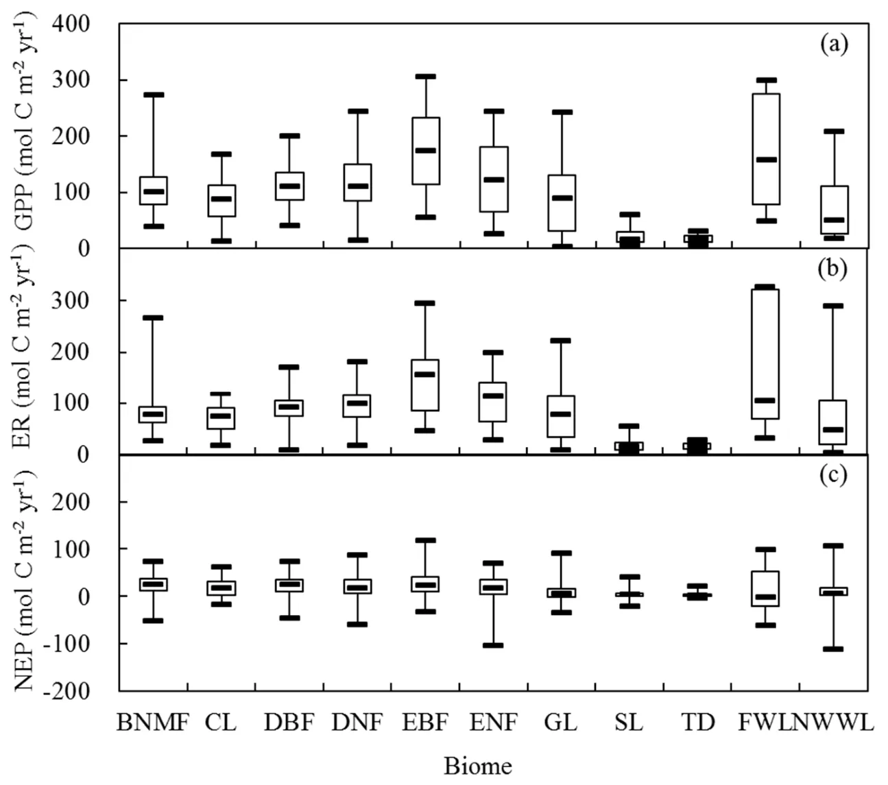
Fig.2.Box-and-whisker plots for Cf luxes:(a)global GPP;(b)ER;(c)NEP.

As indicated in the box-and-whisker plots(Fig.3),the distribution of annual NEP showed clear patterns with the changing climate classes.These results indicated that MAT and MAP inf luence the C f lux component processes di f f erently.The median of NEPdeclined with the increase in the MAT scale when AP was scarce(<0.4 m).However,NEP increased with the increase in MAT when AP ranged from 0.4 to 1.5 m.Themaximum NEPappeared in the MATrange of 10◦C–20◦C when APwas plentiful(>1.5 m).Across the 12 climate classes,the maximum NEP appeared at the upper end of the MATscale(MAT>20◦C)and in themoderate part of the APscale(0.8 m20◦C)and APscale(AP>1.5 m).For all levels of precipitation zones(<0.4m;0.4–0.8 m;0.8–1.5 m;>1.5m),the median of GPPgenerally increased with the increase in MAT[Table S1 in electronic supplementary material B(ESM B)].A similar phenomenon could be seen for the median of ER(ESM B,Table S1),although the tendency was not as obviousasfor GPP.

3.2. Drivers of GPP

Annual GPPexhibited strong relationships with climate factors.For all biomes,GPPwas positively related to MAT and AP(Figs.4aand b).About 17.6%and 32.7%of thevariations in GPP could be explained by MAT and AP,respectively.The relationship between GPPand MAT was f itted by an exponential equation.GPP increased exponentially with the increase in MAT for both non-wetland and wetland(i.e.,FWL and NWWL)biomes(Figs.4d and g).Compared with temperature,precipitation had astronger correlationwith GPPfor non-wetland biomes.APexplained 42.9%of the variability in GPPfor non-wetland biomes(Fig.4e).

GPP was also strongly correlated with LAI(Fig.4c).LAIwas an important factor determining GPPfor both nonwetland and wetland(i.e.,FWL and NWWL)biomes,explaining 34.5%(P<0.001)and 74.6%(P<0.001)of the variability,respectively.For all biomes,LAIexplained 40.2%of the variability in GPP.For wetland(i.e.,FWL and NWWL),GPP was signif icantly correlated to MAT and LAI(Figs.4g and i);GPP was not signif icantly correlated with APin this ecosystem(Fig.4h).

3.3.Driversof ER

Similar to GPP,ER responded to a suite of drivers,including temperature,precipitation and vegetation productivity(Fig.5).In the univariate regressions,MAT,APand LAI were the site-specif ic variables that correlated most strongly with ER.For all biomes,19.1%,32.4%and 33.2%of the variationsin ERcould beexplained by MAT,APand LAI,respectively(Figs.5a–c).Ecosystemswith higher temperature,precipitation and LAI had a larger value of ER as C output.For wetland(i.e.,FWL and NWWL),the drivers of ERwere MAT and LAI(Figs.5g and i);ERdid not exhibit clear precipitation dependency in this ecosystem(Fig 5h).Similar to GPP,ERwas also not signif icantly correlated with soil properties(ESM A,Table S1).The relation between annual ER and GPP is shown in Fig.6.The slope of the relation was 0.805 for all biomes,0.767 for non-wetland,and 1.140 for wetland(i.e.,FWL and NWWL)(intercepts of 4.903,7.847 and−11.498 mol Cm−2per year,respectively).The ER/GPP ratio averaged 0.805 across all sites and years,with values greater than 1(i.e.,net loss of CO2)for wetland(i.e.,FWL and NWWL).

Fig.3.Box-and-whisker plotsfor Cf luxesat di f f erent MATand APscales.Themedian valuesof NEP areshown abovethe NEPplot.

3.4.Driversof NEP

Annual NEPwas weakly correlated with climate factors(i.e.,MAT and AP)(Figs.7a,b,d,e,g and h).Similar to GPP and ER,NEP was signif icantly(P<0.001)correlated with LAIwhen all biomes(Fig.7c)and non-wetland(Fig.7f)were examined.No signif icant correlation between NEPand LAIwasfound for wetland(i.e.,FWL and NWWL)(Fig.7i).Although the R2for the function explaining the relationship between NEPand LAI was relatively low(R2=0.106),the number of independent data points for the f itting was large,ensuring the reliability of the regression function.Moreover,annual NEPwas signif icantly correlated with GPP(ESM B,Fig.S1).The slope of the relation was 0.195 for all biomes,0.234 for non-wetland,and−0.140 for wetland(i.e.,FWL and NWWL).Annual NEPincreased withtheincreasein GPP for non-wetland,and decreased with the increase in GPP for wetland(i.e.,FWL and NWWL).

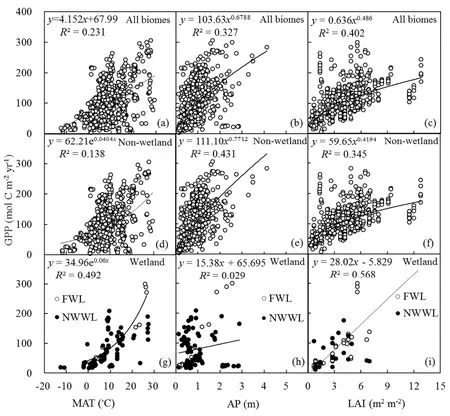
Fig.4.Relationship between GPPand environmental variables:(a–c)MAT,APand LAI,respectively,for all biomes;(d–f)MAT,APand LAI,respectively,for non-wetland sites;(g–i)MAT,APand LAI,respectively,for wetland sites.The P valuesin all panels are less than 0.001.

NEP in our dataset varied with measurement period across the global 24-year C f luxes measurements(ESM B,Fig.S2).A quadratic function could explain the relationship between GPP(or NEP)and measurement period,suggesting the interannual variability of the GPP(or NEP).NEP during the 1993–97 and 2009–14 time periodswaslessthan that during other timeperiods(ESM B,Fig.S3).

NEP at some multiple-year f lux sites showed considerable variability when the interannual variation of NEP was considered.NEP could be quite high in the f irst few years after a long dry period,and then became quite low or neutral even though MAT and APdid not changemuch for afew yearsafter thelong dry period(ESM A,Table S1).Therepresentativesitesthat had such phenomenon were Qianyanzhou(China),Duke forest(USA),Turkey Point(Canada),Pellston(USA),Prince Albert(Canada),Hyyti¨al¨a(Finland),Albuquerque(USA),Dresden(Germany),and Twitchell(USA)(ESM A,Table S1).Plants might show marked responses to increasing precipitation after a long dry period,which could be explained as priming e f f ects.After the dry and humid period,the priming e f f ects of plants to changing precipitation might not be obvious,because plants have acclimatized to theprecipitation f luctuation.

3.5.Modeling GPP,ERand NEP

Therelativecontribution of MAT,APand LAIto each C f lux is indicated in Table S2(ESM B).For the non-wetland,therelativecontribution of APto GPP/ER/NEPin theclimate factor–based model was higher than that of MAT,while the relative contribution of LAIto GPP/ER/NEPin the climateand LAI-based model washigher than that of both MAT and AP.For thewetland(i.e.,FWL and NWWL),therelativecontribution of MAT to GPP/ER/NEP was higher than that of both APand LAI.

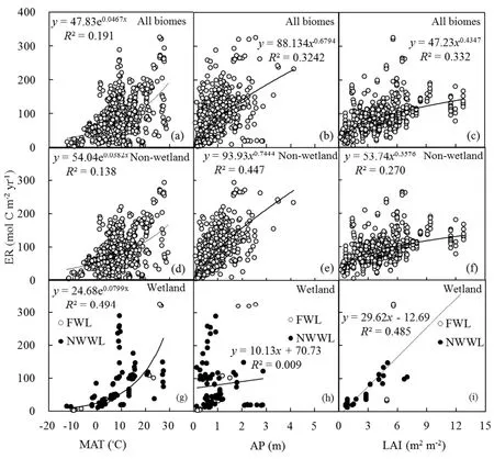
Fig.5.Relationship between ERand environmental variables:(a–c)MAT,APand LAI,respectively,in all biomes;(d–f)MAT,APand LAI,respectively,for non-wetland sites;(g–i)MAT,APand LAI,respectively,for wetland sites.The P valuesin all panels are less than 0.001.

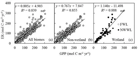
Fig.6.Relationship between ERand GPP:(a)all biomes;(b)non-wetland;(c)wetland.The P valuesin all panels are less than 0.001.

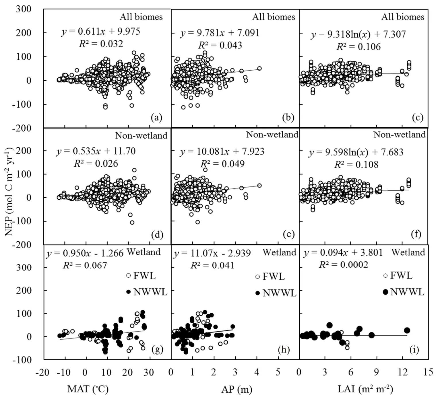
Fig.7.Relationship between NEPand environmental variables:(a–c)MAT,APand LAI,respectively,in all biomes;(d–f)MAT,APand LAI,respectively,for non-wetland sites;(g–i)MAT,APand LAI,respectively,for wetland sites.The P values in(a–f)arelessthan 0.001;the P valuesin(g–i)are0.003,0.019,and 0.921,respectively.

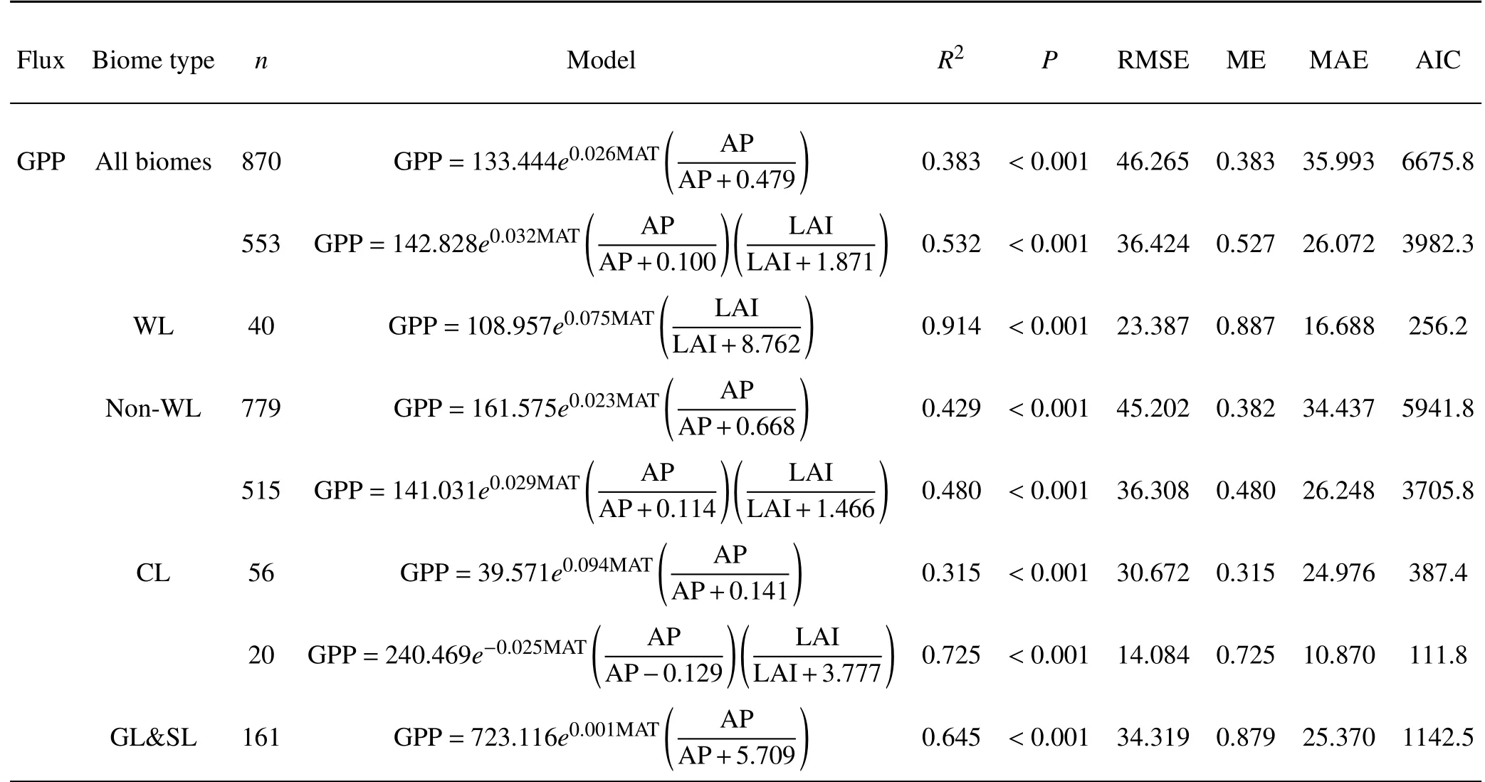
Table 2.Models simulating the inter-site and interannual variability in GPP,ERand NEP(mol Cm−2 yr−1).

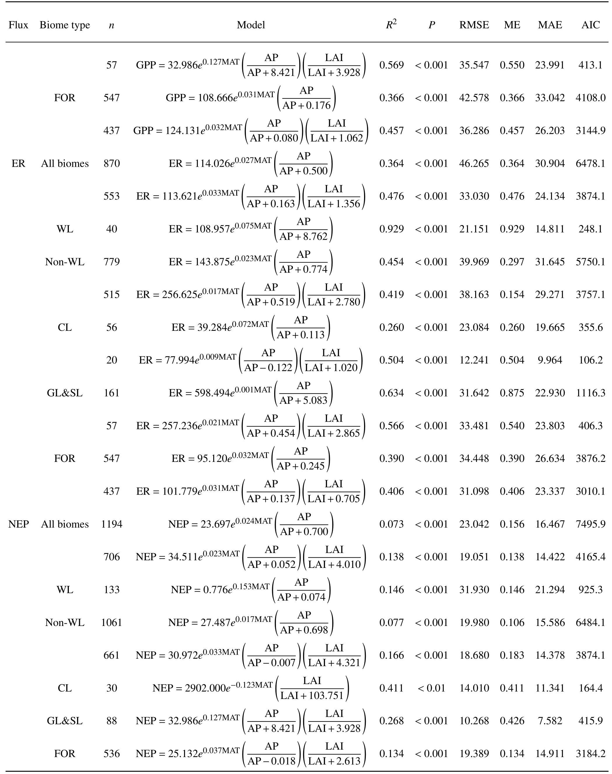
Table 2.(Continued)

Themodelsincluding climatefactorsand LAIareshown in Table 2.For all biomes,the climate factor model named MAT&AP-model explained 38.3%of variations in GPP.The combined contribution of MAT and AP to the spatial and temporal variationsin GPPincreased signif icantly compared with the single-factor contribution of MAT or AP(Fig.4 and Table 2).For all biomes,the RMSE,ME,and MAE for the climate-based GPPmodel were 46.265 mol C m−2yr−1,0.383,and 35.993 mol C m−2yr−1,respectively.For nonwetland,the climate factor model explained 42.9%of variations in GPP.Statistical analyses indicated that the climateand LAI-based model named MAT&AP&LAI-model performed well in simulating the temporal and spatial variability in GPPacross various biomes(Table 2).The model f it of GPP of the climate-based equation related to MAT and AP was improved when the LAIwas incorporated into the model,suggesting that GPP increases with increasing LAI.For all biomes,MAT&AP&LAI-model appeared to be the best f it for the variations in GPPwhen the statistical measures of n,R2,P,RMSE,ME,MAEand AIC were comprehensively evaluated(Table 2).Moreover,for FWL and NWWL,the f it of MAT&LAI-model for GPPhad high values of R2(0.914)and ME(0.887)and low valuesof RMSE(23.387)and MAE(16.688),suggesting that they strongly explain thevariations in GPP.

The climate factor model named MAT&AP-model explained 36.4%of variations in ER.The RMSE,ME,and MAE for the climate-based ER model were 46.265 mol C m−2yr−1,0.364,and 30.904 mol C m−2yr−1,respectively.For non-wetland,the climate factor model explained 45.4%of variations in ER.By integrating the interaction between climate and LAI,the explanation of the regression equation with respect to ER also increased in comparison with MAT&AP-model,when the statistical measures of n,R2,P,RMSE,ME,MAE and AIC were comprehensively evaluated(Table 2).Moreover,for FWL and NWWL,MAT&APmodel explained 92.9%(R2=0.929)of the variations in ER,with low valuesof RMSE(21.151 mol Cm−2yr−1)and MAE(14.811 mol C m−2yr−1).

Compared with GPPand ER,MAT&AP-model explained a lower proportion of the variability in NEP for FWL and NWWL.For all biomes,the RMSE,ME,and MAE for the climate-based NEP model were 23.042 mol C m−2yr−1,0.156,and 16.467 mol C m−2yr−1,respectively(Table 2).The climate factor model explained 7.7%and 14.6%of the variations in NEP for non-wetland and wetland(i.e.,FWL and NWWL).

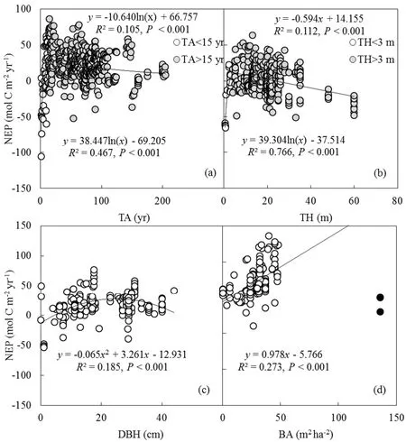
To explore thee f f ectsof land use or disturbance(i.e.,TA,TH,DBH and BA)on NEP,we further examined the relationship between NEP and these variables(Figs.8a–d).As shown in Fig.8a,NEP increased signif icantly(P<0.001)with the increase in TA when TA was less than 15 yr.However,NEPdeclined signif icantly(P<0.001)with theincrease in TA when TA was more than 15 yr,indicating that young trees aged from 10 to 20 yr can absorb more C from the atmosphere.Similar to TA,the trees with height ranging from 10 to 20 m had the highest ability to absorb C.The relationship between NEP and DBH could be well explained by a quadratic model,with adetermination coe f fi cient of 0.185.

Moreover,with over 1000 annual observations for each of those three f luxes from about 300 stations,a number of sites had multiple-year observations.In our analysis,multiple observations from one station were treated as independent observations.Therefore,both inter-site and interannual variations in C f luxes could be determined and modeled.If the multiple-year observations from one station were considered as one sample and modeled on the basis of the averaged multiple-year f luxes and multiple-year environmental variables at each site,the relationship between C f luxes and environmental variables on the basis of integrated site-year data(ESM B,Fig.S4)was similar to that on the basis of all inter-siteand interannual data(Figs.4,5 and 7).

4. Discussion

4.1.Climatecontrol of ecosystem CO2 f luxes

APwasthemost important factor controlling annual GPP and ER across non-wetland biomes.Compared with temperature,precipitation explained a higher proportion of the variance in GPPand ER.The univariate regressions indicated thatprecipitationexplained 42.9%of thevariationsin GPP and 44.6%of the variations in ER for non-wetland(Figs.4e and 5e).Temperature was another important climatic factor controlling the variability in GPP and ER.Overall,warmer and wetter sites had higher GPPand ER,while drier and/or colder siteshad lower GPPand ER.

The relationship between GPP(or ER)and climate factors has been reported by a number of regional and global studies(Law et al.,2002;Kato and Tang,2008;Chen et al.,2013;Reichstein et al.,2013;Yu et al.,2013;Xiao et al.,2013;Xu et al.,2014).For instance,Chen et al.(2013)reported that the combined e f f ects of MAT and AP accounted for 85%and 81%of the spatial variations in GPP and ER in the Asian region,respectively.Xu et al.(2014)examined the global patterns and environmental controls of forest Cbalance,and found that both production and respiration increased with MAT and exhibited unimodal patterns along a gradient of precipitation.For wetland(i.e.,FWL and NWWL),only MATwasresponsiblefor thespatial and temporal variations in GPPand ER.AP was not signif icantly correlated with annual GPPand ER,as water isnot the common limitation to vegetation growth in wetland.

Our study showed that NEPwas signif icantly correlated with MAT and AP(Fig.7),which was in agreement with the results of some regional studies showing that higher air temperature and/or precipitation can lead to higher net C uptake(Yu et al.,2013;Xiao et al.,2013).Chen et al.(2013)reported that MAT and APexplained 36%of the variations in NEP in Asian ecosystems.Annual NEP was also found to be positively related to annual temperature and precipitation in Chinese terrestrial ecosystems(Xiao et al.,2013).Moreover,studieshave shown that climatevariation can be directly responsiblefor short-but not long-termvariation in forest–atmosphere C exchange(Richardson et al.,2007).At global scales,our study showed thatexplaining NEPvariability only viaclimatic variables is ine f f ective.

In this study,precipitation was used as a proxy of water availability.Although precipitation isrelevant,other proxies(e.g.,evapotranspiration,dryness,soil moisture)arealsorelevant.Yiet al.(2010)showed that NEPwasgenerally afunction of temperature at colder sites,relative to a function of drynessat warmer sites.Thissuggeststhat NEPis controlled by a complex interaction of climate factors(i.e.,temperature and dryness).Models incorporating soil moisture perform di f f erently to models using precipitation when simulating soil Cf luxes(McGuireet al.,2000;Exbrayat et al.,2013;Chen et al.,2014;Hursh et al.,2017).Although factors relevant to the relationship between precipitation,dryness and soil moisture are di f fi cult to disentangle at broad scales,temperature and soil texture are thought to be the potential key drivers(Davidson et al.,2000).Addressing this relationship requires more measurement data across a larger number of site-years.Long-term observations of GPP,ER and NEPin various climate zones are needed to verify their variability at di f f erent time scalesand in di f f erent regions.

4.2.Vegetation control of ecosystem CO2 f luxes

Vegetation drivers have been shown to be critical to the inter-site and interannual variations in C f luxes(Jung et al.,2011).In the present study,LAI was an important factor determining GPP and ER for both non-wetland and wetland(i.e.,FWL and NWWL)biomes.Previously,few investigations have reported the correlation between annual GPP and LAI(Luyssaert et al.,2007).On an annual basis,Law et al.(2002)found a poor correlation between GPP and LAI,possibly because the amount of data points was limited in their study.Indeed,LAI is a unique biophysical factor accounting for the di f f erences in phenological development,assimilation and biomass growth in plant canopies(Schmitt et al.,2010).Leaf area exerts a major inf luence on canopy photosynthesis(Tappeiner and Cernusca,1996;Saigusaet al.,1998;Restrepo-Coupeet al.,2013;Wu et al.,2016;Baldocchiet al.,2018),which also provides assimilates for the respiration of roots and soil microorganisms(Reichstein et al.,2003;Bahn et al.,2008,2009;Bond-Lamberty and Thomson,2010).By testing the pairwise relationship between ER and di f f erent site characteristics,Migliavaccaet al.(2011)found that the ecosystem LAI showed theclosest correlation with ER,and thus LAIwasthe best explanatory variableof the ERvariability.

Besides LAI,modeling and in-situ measurement studies have highlighted the importance of biotic drivers,such as stand age,to spatial patterns of C f luxes(Migliavacca et al.,2011).Substrate supply is thought to be more important than temperatureindetermining ERacross European forests(Janssenset al.,2001).The endogenous processes regulate a large part of the daily variation in terrestrial NEP(de Dioset al.,2012).Moreover,ecosystems under the climate optimum often reach their photosynthetic and respiratory potentials,resulting in thelarger contribution of biological e f f ects(compared with climatee f f ects)to theinterannual variability in NEP(Shao et al.,2015).A number of previous studieshaveshown that NEPisa f f ected by interactionsof microclimate,canopy structure,and thephotosynthetic and respiratory physiology of plants(Flanagan and Johnson,2005;Luyssaert et al.,2007;Schmitt et al.,2010),which is essentially in agreement with our results.

4.3. Implications for modeling the terrestrial Ccycle

MAT&AP-model,MAT&AP&LAI-model,and MAT&LAI-model relied on statistical relations between annual GP/ER/NEP and some key controls(climate or LAI),rather than a complete understanding of the mechanisms involved.It was necessary that these simulations generated the correct order of magnitude of measured values and the general patterns from low to high C f luxes.Although previous studies have employed climate variables to simulate C f luxes(Schmitt et al.,2010;Migliavaccaet al.,2011;Yu et al.,2013;Chen et al.,2015),our models included the most inclusive data points of C f luxes and relevant climate and vegetation variables,increasing the simulation e f fi ciency.These results obtained with the bootstrap estimation of MAT&APmodel and MAT&AP&LAI-Model indicated that the developed model described the GPPand ERfor all biomeswell.

The derived parameterization of MAT&AP&LAI-model recorded in Table 2 may be considered as an optimized parameterization for the application of the model at global scales.One of the main advances introduced by this model formulation istheincorporationof LAIasadriver of the GPP and ER.This variable was necessary to improve the description of both the temporal and spatial dynamics of GPP and ER.In this study,wetland(i.e.,FWL and NWWL)was insensitiveto precipitation,possibility owing to thepresenceof water.For wetland,MAT&LAI-model explained more than 90%of variations in GPPand ER,suggesting MAT and LAI are thetwo main driversof GPPand ER.

However,the models shown in Table 2 are relatively crude and did not vary by more specif ic biome types(i.e.,between EBF,ENF,GL,TD,etc.),in spite of the significant variation in biotic controls that would be expected.The unexplained variability in the multiple regressions indicated that GPP,ER and NEP are probably related to a number of factors,including speciescomposition,vegetation characteristics,and spatial variability in nutrient availability(Bahn et al.,2006;Schmitt et al.,2010).The information about vegetation characteristics other than LAI was limited,making it impossible to incorporate these factors into the model.Moreover,thelack of vegetationdatafor each siteand each year increased the di f fi culties of biome-specif ic modeling.More sophisticated analyses are expected if more such vegetation data become available.

The NEP was relatively constant across all types of biomes(Fig.2c).The low variability in NEP constituted a major reason why its measurement and modeling remained sodi f fi cult.By contrast,GPPand ERshowed greatvariability across biomes,and even across sites and years for a specif ic biome(Figs.2a and b);the variability in GPP and ER was generally in accordance with that in temperature and precipitation.NEPresponded to climatedriverswith relatively low R2(Fig.7).Each biome(from EBFin thetropical areato TD inthefrigid zone)canactasanet Csink(i.e.,NEP>0),while controls on the balance between photosynthesis and respiration varied with sites and time scales.The weather conditionslikedrought,thephenology of plants,and thesupply of decomposable litter or exudates may create temporary C storage or lossin ecosystems(Trumbore,2006).However,we did f ind the climate and vegetation controlson NEP(Figs.7 and 8),providingthecluesfor modeling NEP.Thesimulation e f fi ciency of NEPmay be improved if available site-specif ic vegetation data are enough for a particular biome in the future.

The models simulating the variations in the C f luxes of GPP,ER and NEPvaried at the di f f erent scales of MAT and AP(ESM B,Table S3).LAIwas a key driver of C f luxes of GPP,ERand NEPwhen the MATwasatthescaleof lessthan 10◦C.Theinf luenceof MATon Cf luxeswassignif icantatthe scale of lowest MAT(MAT<10◦C)and least AP(AP<0.4 m).APwasoneof thekey driversof Cf luxesof GPP,ERand NEPfrom thesemiarid to-rainy zones(0.4 m

Further analysis using Pearson’s correlation coe f fi cient suggested that maximum C f luxes of GPPmax,ERmaxand NEPmaxover the growing season were signif icantly(P<0.001)correlated with climate factors(MAT and AP)(ESM B,Table S4).The variations in GPPmaxand NEPmaxwere controlled by LAI,while the variations in ERmaxwere not signif icantly(P>0.05)correlated with LAI.MAT,AP and LAI signif icantly(P<0.001)inf luenced the variations in GSL,and GSL was signif icantly(P<0.001)correlated with annual C f luxes(GPP,ER and NEP).Overall,the maximum C f luxes,annual Cf luxes,GSL and climate factors had close relationships.

In our study,ER was strongly correlated with GPP,which could be validated by a number of studies at di f f erent spatial and temporal scales(Lasslop et al.,2010).Larsen et al.(2007)observed that ER depended strongly on photosynthesis in a temperate heath.Janssenset al.(2001)and Reichstein et al.(2007)reported that the annual ER increased linearly with GPPacross European forests.Yu et al.(2013)found that the spatial patterns of GPP and ER of all terrestrial ecosystemsin Chinashowed apositivecorrelation.Thespatial and temporal variationsin ERand GPPwerealso coupled when this analysis was expanded to global ecosystems(Chen et al.,2015).Overall,thistightcoupling conf irms that the variation in photosynthate availability is the dominant driver of respiration and the coupling of GPP and ER should betaken into account in terrestrial Ccyclemodels.

5.Conclusions

Our study provides new insights into the drivers of the interannual and inter-site variability of NEP,GPP and ER.Across terrestrial biomes,climate factorswerefound to play an important role in determining the GPPand ER.For nonwetland,GPPand ER tended to increase towards a warmer and wetter environment.For wetland(i.e.,FWL and NWWL),higher GPPand ER appeared in warmer conditions,whileprecipitation wasnot thefactor limiting siteproductivity and respiration.Meanwhile,the climaterolesweremediated by thevegetation characteristics,such as LAI.However,climate only showed little impact on the variability in NEP,which was relatively constant across all types of biomes.In addition,the vegetation controls(e.g.,LAI and TA)on NEP provided the clues to model NEP.Overall,the e f f ects of LAI on GPP,ER and NEP indicated that canopy-level measurement iscritical for accurately estimating ecosystem–atmosphere exchange of CO2.Climate and LAI can inf luence C f lux components di f f erently in di f f erent climate regions.This synthesis study highlights that the responses of ecosystem–atmosphereexchangeof CO2to climateand vegetation variationsarecomplex,which poses great challenges to models seeking to represent terrestrial ecosystem responsesto climatic variation.

Fig.8.Relationship between NEPand tree characteristics(TA,TH,DBH and BA)due to land use or disturbance:(a)TA;(b)TH;(c)DBH;(d)BA.The several black outliersare not used for establishing the regression line in panel(d).The P values in all panels are less than 0.001.

Acknowledgements.This study was f inancially supported by the National Natural Science Foundation of China(Grant Nos.41775151,41530533 and 41775152).Thousands of researchers who measured the C f lux data collected here contributed greatly to this study.Their f ield measurement work is the basis of this global synthesis.Wearegrateful to thetwo anonymousreviewersfor their helpful commentson our earlier draft.

Electronic supplementary material. Supplementary material is available in the online version of this article at https://doi.org/10.1007/s00376-019-8194-y.