An Adjoint-Free CNOP–4DVar Hybrid Method for Identifying Sensitive Areasin Targeted Observations:Method Formulation and Preliminary Evaluation

Xiangjun TIAN and Xiaobing FENG

1ICCES,Instituteof Atmospheric Physics,Chinese Academy of Sciences,Beijing 100029,China

2University of Chinese Academy of Sciences,Beijing 100049,China

3Collaborative Innovation Center on Forecast and Evaluation of Meteorological Disasters,Nanjing University of Information Science and Technology,Nanjing,210044 China

4Department of Mathematics,University of Tennessee,Knoxville,TN 37996,USA

ABSTRACTThis paper proposes a hybrid method,called CNOP–4DVar,for the identif ication of sensitive areas in targeted observations,which takes the advantages of both the conditional nonlinear optimal perturbation(CNOP)and four-dimensional variational assimilation(4DVar)methods.The proposed CNOP–4DVar method is capable of capturing the most sensitive initial perturbation(IP),which causes the greatest perturbation growth at the time of verif ication;it can also identify sensitive areas by evaluating their assimilation e f f ects for eliminating the most sensitive IP.To alleviate the dependence of the CNOP–4DVar method on the adjoint model,which is inherited from the adjoint-based approach,we utilized two adjointfree methods,NLS-CNOPand NLS-4DVar,to solve the CNOP and 4DVar sub-problems,respectively.A comprehensive performance evaluation for the proposed CNOP–4DVar method and its comparison with the CNOPand CNOP–ensemble transform Kalman f ilter(ETKF)methods based on 10 000 observing system simulation experiments on the shallow-water equation model are also provided.The experimental results show that the proposed CNOP–4DVar method performs better than the CNOP–ETKFmethod and substantially better than the CNOPmethod.

Key words:CNOP,4DVar,NLS-4DVar,targeted observations,sensitiveareaidentif ication

1.Introduction

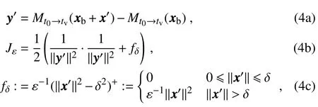
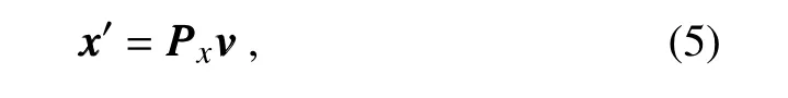
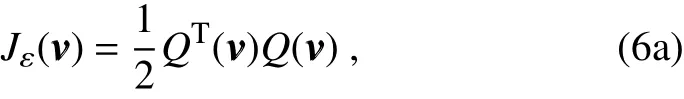
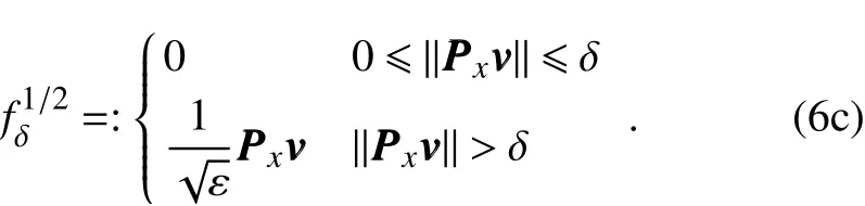
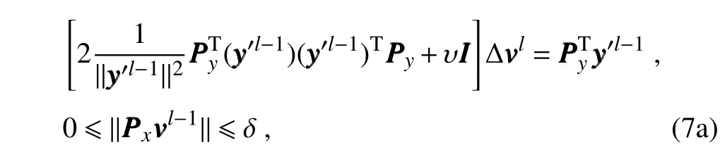
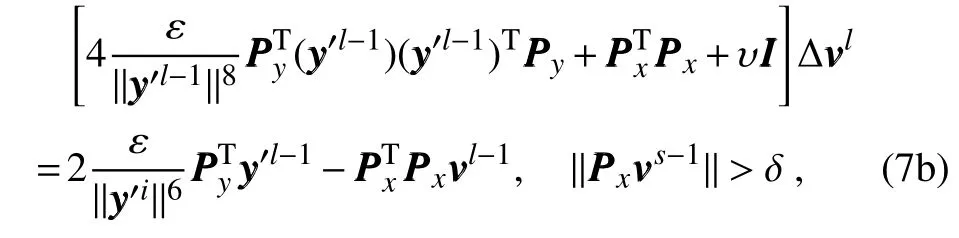
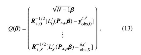
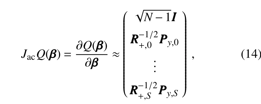
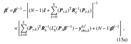
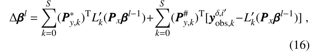
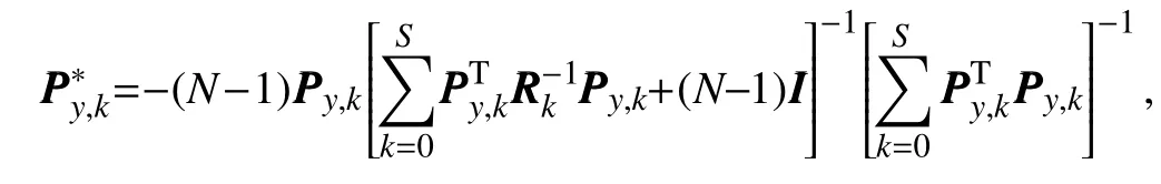
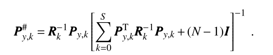
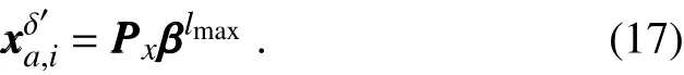
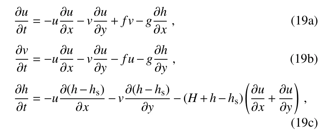
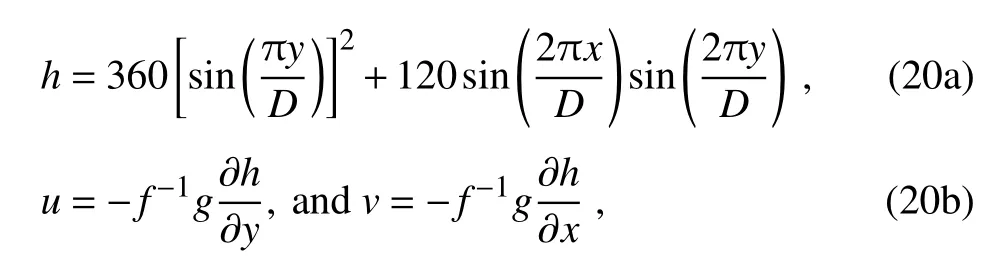
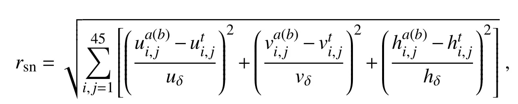
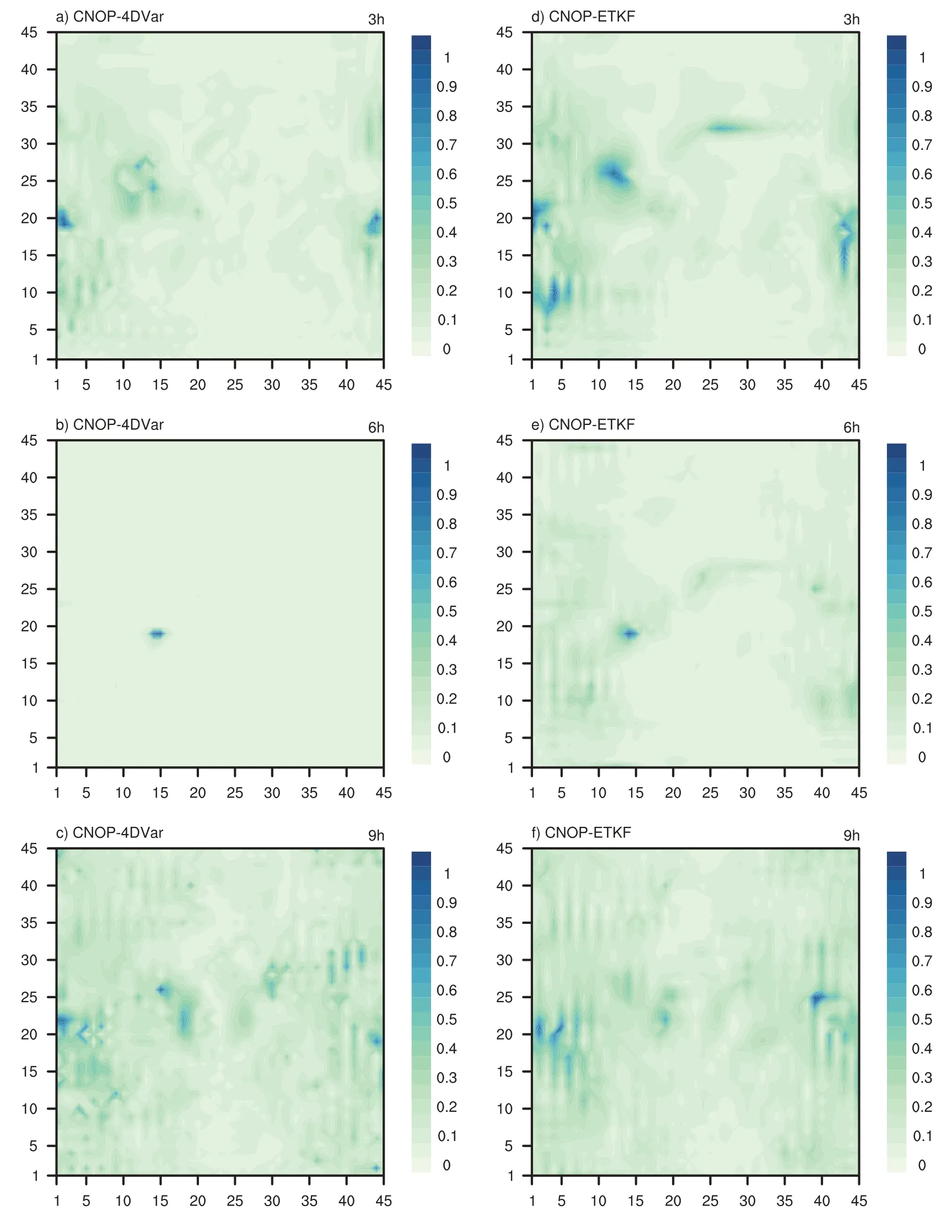
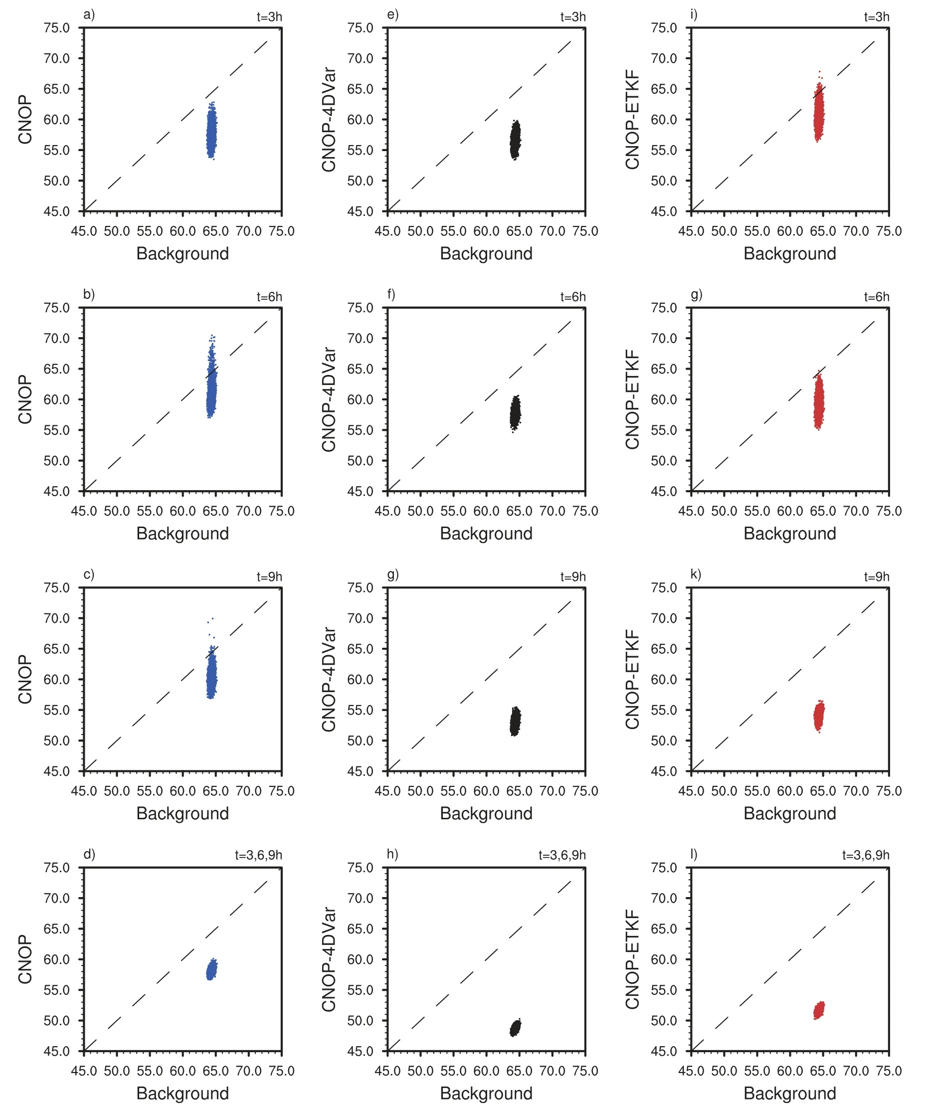
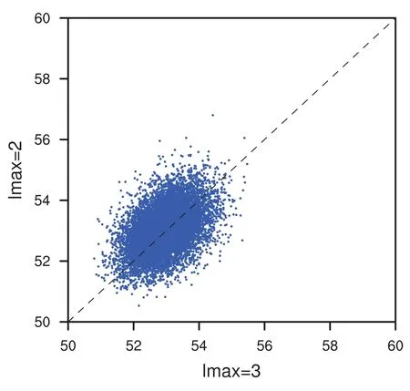
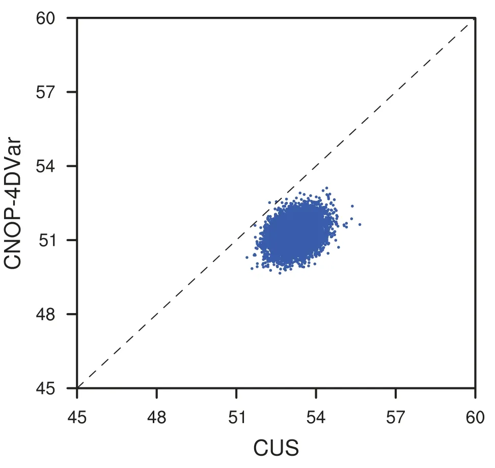
The inclusion of a large amount of observation data into numerical weather prediction(NWP)modelsby dataassimilation has become increasingly vital for accurately modeling high-impact weather events(HWEs)(Joly et al.,1997,1999;Langland et al.,1999a,b,Aberson,2003;Wu et al.,2007a;Aberson et al.,2011;Chou et al.,2011).On the other hand,acquiring su f fi ciently dense f ield observations to fully cover the vast(spatial)areas of HWEs is prohibitively expensive(Mu,2013).To circumvent the dilemma,a targeted(or adaptive)observation strategy was proposed to obtain a limited strategy has been considered as a signif icant contribution to thef ield of weather forecasting.Recall that,to better predict an event at a future verif ication time tv,the idea of targeted observationsisto makeadditional observationsat aproceedingfuturetargettime ta(ta

Existing methods for identifying sensitive areas in targeted observations can be divided into two groups.The f irst group of methodsaimsat capturing themost sensitiveinitial errors,which have the greatest inf luence on prediction accuracy.Areas containing a high concentration of the most sensitive initial errors are identif ied as sensitive areas by these methods.Examples of the f irst group of methods include the quasi-inverse linear method(Pu et al.,1997),the linear singular vector(LSV;Palmer et al.,1998),thesensitivity vector(Langland and Rohaly,1996),ensemble sensitivity methods(Ancell and Hakim,2007),and the conditional nonlinear optimal perturbation(CNOP)method(Mu et al.,2003).In particular,CNOP extends the LSV into a nonlinear regime by overcoming the limitations associated with the linearity assumption in the LSV and obtains promising targeted observation results(Mu et al.,2009;Zhou and Mu,2011).The second group of methods aims at directly reducing prediction uncertainty by assimilating observations throughout all possible observation areas(e.g.Bishop and Toth,1999;Bishop et al.,2001;Daescu and Navon,2004;Hossen et al.,2012;Zhang et al.,2016).These methods compare the error reductions in all possible observation areas based on the extent of the decrease in the forecast error variance in each area,and regard the areas with the greatest assimilation corrections as sensitive areas.Among the methods in the second group,ensemble Kalman f ilter–based methodshavebeen widely adopted due to their implementation simplicity and low computational cost.On the other hand,these methods wereformulated under thelinearity assumption,which limits their applicability to general nonlinear NWPmodels.

It isconcluded that thef irst group of methodsfocusesonly on initial errors;they do not consider the relationships between thoseerrorsand the observations aswell asthe impact of thedataassimilation methodsused.On theother hand,the second group of methodsdonotspecif ically takeinitial errors into consideration.

It seems a natural idea is to combine the two groups of methods to take the advantages of both types while avoiding their def iciencies.Indeed,the need for developing such methods has already been noticed(Mu,2013).The primary objective of this paper is to attempt to meet the need and to f ill the void of missing such methods.Specif ically,we propose a CNOP–4DVar(four-dimensional variational)hybrid method to identify sensitive areas in targeted observations.In this hybrid method,we f irst compute the CNOP xxx′δ∈Rmx(where mxis the dimension of the vector xxx′δand the superscript‘′’denotes the perturbation)of the background state xxxb∈Rmxfor the verif ication time tvand utilize xxxb+xxx′δas the most deviant“true”initial f ield to initialize theforecast model,and to obtain the most deviant“true”model integrations and thepossiblecorrespondingobservations.Wethen adopt a 4DVar-based approach(Rabier et al.,2000)to determine the sensitiveareasby utilizing thepossibleobservationsobtained in the f irst step.An important advantage of the proposed hybrid approach is that it can handle both linear and nonlinear modelsbecause both 4DVar and CNOPare based on nonlinear optimization formulations.Moreover,it is clear that this CNOP–4DVar method can organically integrate errors from all three(i.e.,the initial,target and verif ication)stages into the overall system.Moreover,the proposed hybrid method also has a modular property,which makes the method easily expandable.For example,the 4DVar component in the method may be replaced by the ensemble transform Kalman f ilter(ETKF)method(Bishop et al.,2001),which then results in a new hybrid CNOP–ETKF method for identifying sensitiveareasin targeted observations.

From the def inition it is clear that the proposed hybrid CNOP–4DVar method comprises two nonlinear optimization sub-problems—namely,the CNOPand 4DVar problems.The default approach for solving these sub-problems is the adjoint-based approach.However,it is well-known that developing and maintaining the adjoint model is computationally very expensive.Moreover,the adjoint model is often di f fi cult to obtain when the forecast model is highly nonlinear and/or when the model physics involve discontinuous parameters(Xu,1996).It is well understood that requiring the use of an adjoint model has seriously limited the broader applicability of adjoint-based methods(Tian et al.,2008,2010,2011,2016,2018;Tian and Feng,2015,2017).To alleviate the dependence of using an adjoint model,several ensemble-based approacheshaverecently beendeveloped for the CNOPand 4DVar problems.Among them,the nonlinear least-squares(NLS)–based ensemble method with a penalty strategy for the CNOPproblem(NLS-CNOP;Tian et al.,2016;Tian and Feng,2017)and the NLS-4DVar method for the 4DVar problems(Tian et al.,2011,2018;Tian and Feng,2015)have shown promising and competitive performance due to their implementation simplicity,high accuracy,and lack of dependence on tangent and adjoint models.Both methodswill beemployed to solvethe CNOPand 4DVar subproblemsin the proposed hybrid CNOP–4DVar method.

The rest of this paper is organized as follows:In Section 2,we present our CNOP–4DVar hybrid formulation for identifying sensitive areas in targeted observations.Mathematically,it is adoubleconstrained optimization problem.In section 3,we introduce ensemble-based NLS(adjoint-free)solvers/algorithms for solving the CNOP and 4DVar subproblems in the CNOP–4DVar hybrid formulation;together they give rise to a hybrid CNOP–4DVar method for solving the problem of identifying sensitive areas.In section 4,we present a comprehensiveperformance evaluation for the proposed CNOP–4DVar method and compare it with the CNOP and CNOP–ETKF methods based on 10 000 observing system simulation experiments(OSSEs)on the shallow-water equation model.Finally,we close the paper with a summary and concluding remarksin section 5.

2.The CNOP–4DVar hybrid formulation for theproblem of identifying sensitiveareas

The targeted(or adaptive)observation strategy involves obtaining a limited number of observations distributed over sensitiveareas,whereahigh concentration of themost sensitive initial errors occurs.

Its key idea is to make additional observations at a proceeding future target time ta(ta

where Mt0→tvisthe nonlinear prediction model from t0to tv,xxx′is an initial perturbation(IP)superposed on xxxb,∥xxx′∥δ is the constraint on the IP with∥·∥denoting a given norm,andδis a positive constant(Mu et al.,2003).Qin and Mu(2011)described how to chooseδand to scale the multivariate variables appropriately in real numerical models.Mu et al.(2003)demonstrated thatthe CNOP xxx′δgrowsfaster than other typesof perturbations(including thosebetween the true and background states)due to the dynamic and physical mechanismsof HWEs.

Secondly,we def ine xxxb+xxx′δas the most deviant“true”initial f ield and integratetheforecastmodel xxxta=(xxxb+xxx′δ)to produce the corresponding observations∈Rmy,kfor all possibleobservation areasΩi(i=1,···,ns,where nsis the total number of all possible observation areasΩi)at the targeted observation time(s)ta.

Thirdly,we propose to assimilate the above possible observations yyyδ,iobs,kfrom the i th possibleobservation areasΩiby maximizing thefollowing 4DVar objectivefunctional:

where xxx′denotes the perturbation of the background f ield xxxbat t0,thesuperscript‘T’standsfor thematrix transposeoperation,tkdenotesthe target time,my,kis the dimension of the observational vector yyyδ,iobs,k,b isthebackground value,S+1is thetotal number of targeted observation timepointsin theassimilation window,Hkistheobservation operator,and matrices B and Rkarerespectively thebackground and observation error covariancematrices.

Finally,theanalysisincrement xxxδ′a,i(wherethesuperscript δ′denotes xxxδ′a,icorresponding to xxx′δ)for the i th possibleobservation areaΩiis obtained as the maximizer of E(xxx′)and the areas with the highest concentrations of analysis increment indexesµi′and 0µi1)are designated as sensitiveareas.

3.Ensemble-based NLS algorithm for the CNOP–4DVar formulation

The above proposed CNOP–4DVar formulation for the problem of identifying sensitive area contains two optimization sub-problems,which must be solved numerically to implement the formulation.Solving these optimization problemscould bevery expensiveif theadjoint-based approach is employed.To circumvent thisdi f fi culty,we proposeto solve theseoptimization sub-problemsby using an ensemble-based NLSapproach developed by Tian and Feng(2015,2017)and Tian et al.(2016).

Specif ically,weproposethefollowing four-step algorithm to solve the problem of identifying sensitive areas for an ensemble-based forecast system based on the CNOP–4DVar formulation:

Step 1:Solve the CNOPproblem using the NLS-CNOP approach.The CNOPproblem(1)is f irst approximated by a sequenceof unconstrained optimizationproblems(UOPs,parameterized by the small positive parameterε)using a novel penalty strategy as follows(see Tian and Feng,2017):

where

in which yyy′∈Rmyand xxx′∗∈Rmxdenoteasolution to UOP(3).It can be shown that for a small enoughεthe solution xxx′∗of UOP(3)is a close approximation to the solution xxx′δof the CNOPproblem(1).Wenotethatthisprocedureonly guaranteesf inding one solution to CNOP(1),even if it has multiple solutions(Tian and Feng,2017),and the computed solution is determined by the starting value of the iterative method used to solvethenonlinear problem.

Following the usual ensemble-based approach(e.g.,Tian et al.,2016),we begin by preparing an ensemble of N linearly independent IPs(xxx′j,j=1,···,N)and their corresponding prediction increments(yyy′j=Mt0→tv(xxxb+xxx′j)−Mt0→tv(xxxb),j=1,···,N)at time tv.Assume that any IP xxx′can be expressed by the linear combination of the sampling IPs(xxx′j,j=1,···,N),i.e.:

where PPPx=(xxx′1,···,xxx′N)and vvv[=(v1,···,vN)T]is the coe f ficient vector of the sampling IPs.

Substituting Eq.(5)into Eq.(3)expressing the cost function in termsof the new control variable vvv yields:

where

and

Thus,we have transferred UOP(3)into the above NLS formulation,which can be solved by using the Gauss–Newton iterative method(Dennisand Schnabel,1996).Before doing that,we f irst need to do some necessary modif ications to guarantee its robustness.Letυbe a small positive number def ined as follows(see Tian and Feng,2017 for further details):

and

for l=1,2,···,lmax(lmaxis the maximum iteration number),where PPPy=and III isan N×N identity matrix.

An e f fi cient localization process is often used in this ensemble-based approach to f ilter out spurious correlations resulting from inadequate sampling or false long-range correlations(Houtekamer and Mitchell,2001).After the localization process is done,the Gauss–Newton iteration(7)can be rewritten as:

and

where

and

Here,ρxρTx=CCC∈Rmx×mxis the spatial correlation matrix(Tian et al.,2016;Zhang and Tian,2018a).ρy∈Rmy×rshould be computed together withρx∈Rmx×r,and r is the selected truncation modenumber(Zhang and Tian,2018a).Consequently,we obtain=+∆vvvlmaxρand xxx′δ=PPPx,ρvvvlmaxρ.Thesubscript‘ρ’represents“localization”.

Step 2:Integratetheforecast model xxxta=Mt0→ta(xxxb+xxx′δ)to obtain the most deviant observationsat the target time(s)ta(=t1,···,tS).

Step 3:Solve the 4DVar problem(2)with observations yyyδ,iobs,kusing the NLS-4DVar.For easeof presentation,wef irst rewrite Eq.(2)asfollows:

where

Similarly,we assume that the analysis increment xxx′can be expressed as a linear combination of the sampling IPs(PPPx);namely,

whereβ[=(β1,···,βN)T]is the vector of coe f fi cients of the sampling IPs.Substituting Eq.(10)and the ensembleestimated BBB≈PPPxPPPTx

N−1(Evensen,1994)into Eq.(9)and expressing the cost function in terms of the new control variableβ yields

Equation(11)can be further rewritten as the following quadratic cost function:

where

where PPPy,k=(yyy′k,1,···,yyy′k,N)and yyy′k,j=Lk(xxxb+xxx′j)−Lk(xxxb).The nonlinear least-squares formulation[Eqs.(12)–(14)]is then solved by the Gauss–Newton iterative method[see

Tian and Feng(2015)and Tian et al.(2018)for further details],as follows:

and therefore,

Following Tian and Feng(2015),we obtain

where

and

The analysis increment for the i th possible observation areaisthusgiven by

Liketheensemble-based approach to the CNOPproblem shown in Step 1,we adapt an e f fi cient localization scheme(Zhang and Tian,2018a)that wasoriginally proposed for the NLS-4DVar by Tian et al.(2018)by transforming Eq.(16)into the following form:

4. Preliminary evaluations using the shallowwater equation model

4.1. Experimental setup

We utilize a two-dimensional(2D)shallow-water equationmodel(Qiu et al.,2007)toevaluatetheproposed CNOP–4DVar hybrid method,particularly in comparison with the CNOPmethod and the CNOP–ETKF hybrid method.The 2D shallow-water equationsaregiven in the f-planeby

where g is the acceleration of gravity,f=7.272×10−5s−1is the Coriolis parameter,H=3000 m is the basic-state depth,hs=h0sin(4πx/Lx)[sin(4πx/Ly)]2istheterrainheight,h0=250 m and D=Lx=Ly=13 200 km are the lengths of thetwo sidesof the computational domain,respectively,and the uniform grid size is taken as d=∆x=∆y=300 km.The computational domain is partitioned into a square mesh with 45 grid points in each coordinate direction and the periodic boundary conditions are imposed at x=0,Lxand y=0,Ly.The spatial/local time derivatives are discretized by the second order central f initedi f f erenceschemeand two-step backward di f f erence scheme of Matsuno(1966),respectively.We choose the time step size∆t=360 s(or 6 min).The model statevector isrepresented by height h and horizontal velocity components u and v at thegrid points.

Similar to Tian and Xie(2012),we prepare the background(initial)state xxxb(Fig.1)by integrating the shallowwater equation model with the imperfect h0=0 m from the following initial conditions(ICs):at t=−60 h for 60 hours.We assume the spatially averaged root-mean-square errors(RMSEs)to be 23.4 m,1.53 m and 2.58 m s−1for the h,u and v f ields,respectively.Theverif ication timeis12 h and thetarget timesare3,6,and 9 h,respectively.Additionally,∥·∥and√ for the CNOP problem.At this stage,we utilized the NLS-CNOP method to compute the CNOP xxx′δof the background state xxxbfor the verif ication time tv=12 h,which in turn determines the CNOP-type sensitive areas.Subsequently,themost deviant observations yyyδ,iobs,kcan bedetermined at the target times(i.e.,ta=3,6 and 9 h)by xxxta=Mt0→ta(xxxb+xxx′δ),where Mt0→tais the shallow-water equation model with h0=250.Thus,we apply the NLS-4DVar and ETKF methods to determine the sensitive areas among all possibleobservation areasΩi(i=1,···,nsand ns=45×45)using the observations yyyδ,iobs,kobtained at the target times.

Fig.1.Spatial distribution of the ICsat 0 h:(a)u(m s−1);(b)v(m s−1)and h(m s−1).

The second part of our numerical experiments involves designing a large number of 4DVar-based OSSEs,by assimilating the synthetic observations in the identif ied sensitive areas.For this purpose,we f irst generate a basic“true”state xxxt,0by integrating theshallow-water equation model with the perfect h0=250 m from the same ICs[see Eq.(20)]for 60 h.Subsequently,10 000 groups of“true”initial states xxxt,s(where the subscript‘s’denotes the s th“true”initial state and s=1,2,···,10000)aregenerated by adding randomconstraint perturbations xxx′t,s(∥xxx′t,s∥δ)to the basic“true”states xxxt,0as xxxt,s=xxxt,0+xxx′t,s.Model-produced“true”f ields at 3,6,9 and 12 h,respectively,are therefore produced after 12-h integrations from the“true”initial xxxt,sat the same starting time in the f irst part of our numerical experiments.The synthetic observationsin the identif ied sensitive areas at the target times(tk=3,6,and 9 h)in the CNOP,CNOP–4DVar and CNOP–ETKFmethods are generated by adding random noise to the model-produced“true”f ields,respectively.The number of observations my,kistaken to be225 for each target time(3,6,and 9 h).

We evaluate the observations in the sensitive areas(consisting of 225 grid points)obtained by the CNOP,CNOP–4DVar and CNOP–ETKF methods using 10 000 4DVarbased OSSEs with the 10 000“true”initial states xxxt,s(s=1,···,10 000)and their corresponding synthetic observations for a single observational time level(i.e.,t0=3,6,or 9 h),and for all three observational time levels[i.e.,tk=3(k+1)h,k=0,1,and 2].The background xxxbis the same as used in the f irst part of our numerical experiments.We then further comparethe CNOP–4DVar observation strategy with the commonly used strategy involving theselection of sparsedata pointsin the observation area.

In addition,wealso usethe NLS-4DVar approach for data assimilation in thesecond part of thenumerical experiments.The standard parameters are an ensemble size N=90 and a covariance localization Schur radius of dh,0=dv,0=10×30 km for all three ensemble-based(NLS-CNOP,NLS-4DVar,and ETKF)methods.

4.2.Experimental results

A comparison of the spatial distribution of the CNOP u′δ[(u′δ,v′δ,h′δ)=xxx′δ]with a verif ication time of 12h,and its corresponding model perturbations u′tk[(u′tk,v′tk,h′tk)=xxx′tkand xxx′tk=Mt0→tk(xxxb+xxx′δ)−Mt0→tk(xxxb)]at thetarget times(tk=3,6,and 9 h)are shown in Fig.2.The locations of areas with ahigh concentration of errorschangewith model integration.Therefore,we check whether the CNOP-determined sensitive areas(at the initial time)perfectly match with those at thetarget times.Weobservethat thesensitiveareasidentif ied by the CNOP–4DVar/ETKFmethodsaresignif icantly di f f erent from those obtained by the CNOP method at all target times(Figs.2 and 3).Furthermore,thereisalargevariability in the CNOP–4DVar/ETKF-determined sensitiveareasatdifferent target times(Figs.3a–c and Figs.3d and e).Moderate di f f erences are also found between the CNOP–4DVar-and CNOP–ETKF-determined sensitive areas,even at the same target times.This is the consequence of using di f f erent optimization methods(i.e.,NLS-4DVar vs ETKF)by the two methodsto identify sensitiveareas.

We then quantitatively examine the performance of the three methods using normalized RMSEs,which are computed by the formula

Fig.2.Spatial distribution of(a)the CNOP u′δ(m s−1)and itscorresponding model perturbations u′tk(ms−1)at(b)3 h,(c)6 h and(d)9 h.

where a,b and t indicatetheassimilated,background and true solutions,respectively.We compare the background-derived RMSEs with the corresponding NLS-4DVar-derived RMSEs by assimilating the observations in the sensitive areas identif ied by the CNOP,CNOP–4DVar and CNOP–ETKFmethods atasingletargeted observationtime(t0=3,6,or 9h),respectively,and at all three target times(tk=3,6,and 9 h).The results show that all three methods are satisfactory in terms of the overall lower RMSEs compared with the backgroundderived RMSEs for the total 10 000 experiments.Generally,if the target time iscloser to the verif ication time,the assimilation performance becomes better;and using multiple target times produces a substantially more accurate result than using a single target time.The proposed CNOP-4DVar hybrid method isthe best performing method among thetested methods.It moderately surpasses the CNOP–ETKF method but substantially outperforms the CNOP method.Presumably,the sensitive areas with high concentrations of errors at theinitial rather than targettimeof the CNOPmethod iscredited for itsinferior performancecompared with theother two methods.The 4DVar nonlinear optimization of the CNOP–4DVar method is superior to the ETKF method adopted by the CNOP–ETKFapproach,leading to lower RMSEsfor the CNOP–4DVar method than for the CNOP–ETKF method,both at oneand threetarget time(s)(Fig.4).

The use of the maximum iteration number lmaxfor the NLS-4DVar solver in Step 3 of the proposed CNOP–4DVar method clearly inf luences to a large extent the computational accuracy and complexity.To determine the inf luence of the number of iterations on the CNOP–4DVar results,we evaluate the CNOP–4DVar-determined sensitive areas at target time ta=9 h with lmax=1,2,3,and 4.As Fig.5 shows,only small di f f erences are observed when lmax2.We also compare RMSEs by assimilating the CNOP–4DVar-determined observations at ta=9 h for lmax=2 and 3;Fig.6 shows that their di f f erences are mainly concentrated near the diagonal line y=x in both cases,which implies that they generally have a similar performance,and that the Gauss–Newton iterative method ensures that NLS-4DVar reaches its minimum after only oneto two iterations,which isalso consistent with theresultsof our previousstudies(Tian and Feng,2015;Tian et al.,2018).

Fig.3.Spatial distribution of the(a–c)CNOP–4DVar-determined and(d–f)CNOP–ETKF-determined analysis increment indexesat(a,d)3 h,(b,e)6 h and(c,f)9 h.

We also compare the proposed CNOP–4DVar method with the commonly used sparse observation strategy,by selecting 225 sparse grid points within the observation area.For the CNOP–4DVar observation strategy,we chose observation points(j=1,···,my,k),in decreasing order ofwith a grid size3×300 km.For the sparse observation strategy,observation points are chosen at sparsely selected grid points equally spaced every 3d=900 km in each coordinate direction.As expected,the proposed CNOP–4DVar hybrid method substantially outperforms the sparse strategy in all 10 000 experiments(Fig.7).The results of these experiments show that the proposed hybrid method is indeed capableof achieving higher assimilation accuracy.

Fig.4.Comparisons between the background-derived RMSEs and the corresponding NLS-4DVar-derived RMSEs by assimilating theobservationsin thesensitiveareasobtained by the(a–d)CNOP,(e–h)CNOP–4DVar,and(i–l)CNOP–ETKFmethods at a singletargeted observation time(t0=3,6,or 9 h),respectively,and at all threetarget times(tk=3,6,and 9 h).

5.Summary and concluding remarks

Fig.5.Spatial distribution of the CNOP–4DVar-determined analysis increment indexes at the single targeted observation time(t0=9 h)for l max=1,2,3,and 4,respectively.

Fig.6.Comparisons between the NLS-4DVar-derived RMSEs by assimilating the observations in the sensitive areas obtained by the CNOP–4DVar method for l max=2 and 3,respectively,at a single targeted observation time(t0=9 h).

Fig.7.Comparisons between the NLS-4DVar-derived RMSEs by assimilating the observations in the sensitive areas obtained by the CNOP–4DVar method and the commonly used strategy(CUS),respectively,at asingletargeted observation time(t0=9 h).

Existing methods for identifying sensitive areas in targeted observations can generally be divided into two groups,according to whether they aim to directly reduce initial errors or prediction errors;these two groups of methods are only weakly linked.In this paper we propose a hybrid method,called the CNOP–4DVar method,which links these two groups of methods and takes the advantages of both the CNOP and the 4DVar method.The proposed CNOP–4DVar hybrid method is capable of capturing the most sensitive IP,which causes the greatest perturbation growth at the time of verif ication,and its 4DVar capability allows it to identify sensitive areas by evaluating their assimilation effectsfor eliminating themost sensitive IP,which hasalready been captured by its CNOP capability.The adjoint-based approach is typically used to solve the CNOP and 4DVar nonlinear optimization problems,but it is computationally very expensive for large-scale problems.To avoid the limitations of the adjoint-based approach,we adopt two adjointfree methods—namely,the NLS-CNOP and NLS-4DVar methods—to solve the CNOPand 4DVar sub-problems,respectively.

Wecarry outacomprehensiveperformanceevaluation for the proposed CNOP–4DVar hybrid method by comparing its results with those obtained by the CNOPand CNOP–ETKF methods over 10 000 OSSEs based on the shallow-water equation.The results show that the proposed CNOP–4DVar method generally performs better than the CNOP–ETKF method,but substantially better than the CNOP method.Compared with the CNOP method,the CNOP–4DVar hybrid method hasan additional advantageof being ableto precisely locate sensitive areas at the target time.Our tests also show that the4DVar-based nonlinear optimization used in the CNOP–4DVar hybrid method issuperior to the ETKFmethod used in the CNOP–ETKFhybrid method.

Step 3 of the CNOP–4DVar hybrid method requires the use of the NLS-4DVar method with lmax≈2,throughout all possibleobservation areas.Admittedly,thisrequirementmay be computationally costly,especially in complicated realworld nonlinear weather and climate models.This issuemay beovercomeand evaluated by themultigrid iterativescheme(Zhang and Tian,2018b)and will bestudied in aforthcoming work.

Acknowledgements.Thework of thef irst author waspartially supported by the National Key R&D Program of China(Grant No.2016YFA0600203)and the National Natural Science Foundation of China(Grant No.41575100).