LASG Global AGCM with a Two-moment Cloud Microphysics Scheme:Energy Balance and Cloud Radiative Forcing Characteristics

Lei WANG,Qing BAO,Wei-Chyung WANG,Yimin LIU,Guo-Xiong WU,Linjiong ZHOU,Jiandong LI,Hua GONG,Guokui NIAN,Jinxiao LI,Xiaocong WANG,2,and Bian HE,2

1State Key Laboratory of Numerical Modeling for Atmospheric Sciences and Geophysical Fluid Dynamics,

Institute of Atmospheric Physics,Chinese Academy of Sciences,Beijing 100029,China

2CASCenter for Excellencein Tibetan Plateau Earth Sciences,Chinese Academy of Sciences,Beijing 100101,China

3College of Earth and Planetary Sciences,University of the Chinese Academy of Sciences,Beijing 100049,China

4Atmospheric Sciences Research Center,State University of New York,Albany,New York 12203,USA

5National Oceanic and Atmospheric Administration,Geophysical Fluid Dynamics Laboratory,Princeton,NJ 08540-6649,USA

ABSTRACT Cloud dominatesinf luencefactorsof atmospheric radiation,whileaerosol–cloud interactionsareof vital importanceinits spatiotemporal distribution.In this study,a two-moment(mass and number)cloud microphysicsscheme,which signif icantly improved the treatment of the coupled processes of aerosols and clouds,was incorporated into version 1.1 of the IAP/LASG global Finite-volume Atmospheric Model(FAMIL1.1).For illustrative purposes,the characteristics of the energy balance and cloud radiative forcing(CRF)in an AMIP-type simulation with prescribed aerosols were compared with those in observational/reanalysisdata.Even within theconstraintsof theprescribed aerosol mass,themodel simulated global mean energy balanceat thetop of theatmosphere(TOA)and at the Earth’s surface,aswell astheir seasonal variation,arein good agreement with the observational data.The maximum deviation terms liein the surface downwelling longwaveradiation and surface latent heat f lux,which are 3.5 W m−2(1%)and 3 W m−2(3.5%),individually.The spatial correlations of the annual TOA net radiation f lux and the net CRF between simulation and observation were around 0.97 and 0.90,respectively.A major weakness is that FAMIL1.1 predicts more liquid water content and less ice water content over most oceans.Detailed comparisons are presented for a number of regions,with a focus on the Asian monsoon region(AMR).The results indicate that FAMIL1.1 well reproducesthe summer–winter contrast for both thegeographical distribution of thelongwave CRFand shortwave CRFover the AMR.Finally,the model bias and possible solutions,aswell as further works to develop FAMIL1.1 are discussed.

Key words:two-moment cloud microphysics scheme,aerosol–cloud interactions,energy balance,cloud radiative forcing,Asian monsoon region

1.Introduction

The formation and evolution of the Earth’s climate system is regulated by spatiotemporal variations in the global energy balance.Clouds play a signif icant role in the Earth’s weather and climate change owing to their inf luences on the transfer of radiative energy,as well as on the spatial distribution of latent heating in the atmosphere.Indeed,a lack of observational data on clouds and related processes has long been amongthemajor sourcesof uncertaintiesin understanding climate change(Bony et al.,2006;Zelinka et al.,2017).Atmospheric aerosols further complicate estimations and interpretations of the changing energy balance in the Earth system,both through their direct e f f ects(transfer of radiative energy)and indirect e f f ects(aerosol–cloud interactions).Aerosol–cloud–climate interactions are of vital importance in climate system models because of the role they play in global and regional energy balancesand cloud radiativeforcing(CRF).Climate modelsis the most commonly used tools for studies on aerosol–climate and aerosol–cloud–radiation interactions(Rosenfeld et al.,2014;Fan et al.,2016).And a comprehensivephysically–based cloud microphysicsscheme is essential to characterize the part played by aerosols in the nature of clouds and the Earth’s climate when investigating aerosol–climateand aerosol–cloud–radiation interactions.

Currently,two types of cloud microphysics schemes are used in climate models:bin microphysics schemes(Feingold et al.,1994;Jiang et al.,2001)and bulk water microphysicsschemes(Lin et al.,1983;Reisner et al.,1998;Hong et al.,2002).Bin microphysics schemes divide the particle size spectrum into di f f erent bins and can directly simulate the evolution of individual hydrometeors and aerosol particles.In contrast,bulk water microphysics schemes mainly consider theoverall spectral distribution of particlesizes,and are therefore suitable for describing the general characteristics of natural cloud precipitation particles(Duan and Mao,2008).Bin schemes are not suitable for long-term experiments(Roh et al.,2017)because they require large amounts of computation time and memory,especially in global-scale high-resolution experiments.Therefore,bulk water microphysics schemes are commonly adopted in climate models with large domains.Bulk water microphysics schemes can befurther subdivided into single-moment and multi-moment schemes on the basis of the number of prognostic variables.The most widely used multi-moment microphysics schemes in climatemodels are two-moment schemes(Morrison et al.,2005;Seifert and Beheng,2006;Lim and Hong,2010).Twomomentmicrophysicsschemesallow greater f lexibility inthe particle size distribution than single-moment schemes and havebeen implemented in many state-of-the-art regional and global climate models,such as the WRF model,the CAM5(Morrison et al.,2005)and the NOAA/GFDL’s Atmospheric General Circulation Model(Salzmann et al.,2010).Previous work hasalso shown thattwo-momentmicrophysicsschemes provide a better representation of the cloud radiative propertiesthan single-moment schemes,leading to a more accurate simulation of the e f f ects of radiative cooling and heating on circulation patterns(Lee and Donner,2011).

The IAP/LASGhasa long history of working on climate model development(Wu et al.,1996;Bao et al.,2010;Li et al.,2013,2014b;Zhou et al.,2015),and thelatest version of its climate system model is called the FGOALS3.The atmospheric component of FGOALS3 is version 1 of the Finitevolume Atmospheric Model of the IAP/LASG(FAMIL1),which began its development in 2011.With a f lexible horizontal resolution of up to 6.25 km,FAMIL1 has been comprehensively evaluated on China’s Tianhe-1 and Tianhe-2 supercomputer,and exhibited an excellent performancein term of the computing speed and e f fi ciency(Zhou et al.,2012;Li et al.,2017b).Zhou et al.(2015)evaluated the energy balance in FAMIL1 and showed that the model performs well in simulations of the annual mean geographical distributions and seasonal cycle of radiative f luxes at the TOA,as well as thelatentand sensibleheatf luxesatthe Earth’ssurface.However,regional deviations still exist in the model.One of the signif icant simulation bias in the energy balance modeled by FAMIL1 can be seen in the eastern oceanic regions.Also,in East Asia—a very important climatic region with large anthropogenic–aerosol loading because of its high levels of industrial and domestic emissions,theaerosol–cloud–climate interactions require further verif ication.However,FAMIL1 usesabulk water microphysicsschemewith asinglemoment(Lin et al.,1983;Harris and Lin,2014)and therefore cannot physically describetheaerosol–cloud interactionsat theprocesslevel at that time.Therefore,in thisstudy,FAMIL1 was coupled with a physically based two-moment,six-class bulk water cloud microphysics scheme(CLR2)(Chen and Liu,2004;Cheng et al.,2007,2010)with the aim to better describetheaerosol–cloud interactionsand relevantmicrophysical processesin anew iteration of themodel,FAMIL1.1.

Using a standardized Atmospheric Model Intercomparison Project(AMIP)experiment with a horizontal resolution of 2◦,the global and regional[focusing on the Asian monsoon region(AMR)]characteristics of the simulated energy balance and CRFin FAMIL1.1 were evaluated.Specif ic aimsof thestudy included:(1)to assessthemodel’s performance in reproducing the global energy balance with CLR2;(2)to identify themain biasesin thesimulated energy balanceand thepossiblereasonsfor them;and(3)to evaluate the model’s performance in reproducing the CRF and cloud macro-physical featuresover the AMR.

Theremainder of thispaper isorganized asfollows.Section 2 describes FAMIL1.1,CLR2,and the experimental design.Section 3 describes the observational and reanalysis data used in the evaluation.Section 4 reports the energy balance and relevant cloud–radiation properties modeled by FAMIL1.1.Finally,asummary of thekey f indingsand some further discussion comprises section 5.

2.Model description and experimental design

2.1.Model description

Thehorizontal resolution of FAMIL1.1 is Cube-sphere48(C48,about 200 km)and the vertical resolution is a 32-layer hybrid vertical grid with amodel top of 2.16 hPa(thevertical height isabout40 km).Mostof thephysical parameterization schemesin FAMIL1.1 arethesameasthoseused in FAMIL1(Zhou et al.,2015),the major update in FAMIL 1.1 is the incorporation of the CLR2,which considers the coupling processes in aerosol–cloud–radiation–climate interactions.In addition,theplanetary boundary layer(PBL)schemewasupdated,from anon-local scheme(Holtslag and Boville,1993)to ahigher order turbulenceclosureschemefrom the University of Washington(Bretherton and Park,2009)to obtain a realistic valuefor theturbulencekinetic energy(TKE),which isrequired to couplethe CLR2.

The CLR2 simulates cloud–aerosol interactions through the activation of cloud droplets from cloud condensation nuclei(CCN)and the restoration of aerosols from the evaporation of cloud droplets.Details of all the microphysical processes in the CLR2 were reported by Cheng et al.(2010).Collaborative research and further development on this scheme were reported by Wang et al.(2017). This schemehaspreviously been coupled to regional climatemodels to investigate the impacts of aerosols on the cloud microphysics,radiative properties of clouds,precipitation,and tropical cyclones,et al.(Cheng et al.,2010;Hazra et al.,2013;Chen et al.,2015,2018;Yang et al.,2018).However,the microphysicsscheme used in regional climatemodels cannot be applied directly in global climate models becauseof“grid-resolution problems”(Wood et al.,2002).For instance,the number of cloud droplets activated at the cloud base shows a strong sensitivity to the saturation excess;and saturation excess is highly dependent upon updraft velocity.However,thegrid-box mean updraft velocity isoften too low and can beeasily averaged out in a GCM with coarseresolution.A sub-grid treatment should be therefore used in GCM to mitigate this problem.In FAMIL1.1,the sub-grid-scale updraft velocity[(Eq.1)]is used to calculate the activation of aerosol particles based on the general theory of isotropy(Pinto,1998):

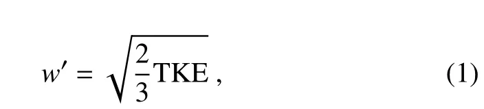
where wis the vertical motion and TKE is the turbulence kinetic energy.

The CFMIPObservation Simulator Package(COSP)has also been coupled online with FAMIL1.1 to provide simulated clouds against the satellite products.COSPis an integrated satellite simulator and enables the conversion of simulation information from model data into several satelliteborne active and passive sensor products,which facilitates the use of satellite data to evaluate a model’s simulation performance in a consistent way.This simulator established a bridgebetween both model–satelliteand model–model intercomparisons(Bodas-Salcedo et al.,2011).

2.2. Experimental design

A standardized AMIP experiment(prescribed SST)was used to evaluate the energy balance and CRF.The easydesigned AMIP-type experiments are regarded as standard testbedsfor theevaluationof thephysicsschemesand enables to focus on the atmospheric model without the added complexity of ocean-atmosphere feedbacks in the climate system.The advantage of an AMIP experiment is that it does not require a long spin-up to achieve model stability.Also,the so-called climate-drift problem in air–sea coupled models can be avoided.However,the absence of air–sea coupling process will a f f ect the simulation for atmospheric circulation over monsoon regions,thus impact the large-scale background for cloud production.Although another air–sea coupled experiment integrated for a long timewas available,AMIPexperimentwasstill used to testtheperformanceof the microphysics scheme in this study.The model(FAMIL1.1),with amonthly output,wasintegrated from 1979 to 2009 and the last nine years(2001–09)simulations were extracted for comparison with the observational and reanalysis data.The averagebackground in the CLR2(Whitby,1978)ischosen to describe the aerosol number density distribution.The mass loading of the prescribed aerosol in FAMIL1.1 was taken from NCAR Community Atmosphere Model with Chemistry(CAM-Chem)(Lamarque et al.,2012),which were the aerosol datarecommended for CMIP5.Based onpreviousreports(Abdul-Razzak and Ghan,2000),external mixing processeswereconsidered intheactivation processesof the CCN activity of sulfate aerosolsand sea-salt aerosols.

3.Datasets

The following data were used to evaluate the simulated energy balance:(1)monthly radiative f lux data from the Cloudsand Earth’s Radiant Energy System–Energy Balanced and Filled(CERES-EBAF)edition 2.8 dataset;(2)monthly surface sensible and latent heat f lux data from the European Centrefor Medium-Range Weather Forecasts(ECMWF)Reanalysis Interim(ERA-Interim)dataset;and(3)monthly cloud water data from the CloudSat 2B-CWC-RO version R04 data product.The horizontal resolutions of the CERESEBAFand ERA-Interim datasets are 2◦×2◦and 1◦×1◦,respectively;both cover the period 2001–09.The CloudSat dataset is remapped from the satellite pixels to the 2.5◦×2.5◦longitude–latitude box,which is the resolution commonly used in previous studies(Sassen and Wang,2008;Ellis et al.,2009).The CloudSat datasets covered the period 2007–11.

4.Results

4.1. Annual global mean energy balance of the Earth

The Earth’s annual global mean energy balance at the TOA and on the surface obtained from FAMIL1.1 are f irstly compared to that from several di f f erent datasets,including satellite products,reanalysis data,and the outputs from the CMIP5 models(Fig.1).Those datasets parallel that of Zhou et al.(2015).The simulated global annual mean radiation f luxes at the TOA and at the Earth’s surface,as well as the heat f luxesat the Earth’ssurface,arein good agreement with theobservations.For example,themaximum deviation terms lie in the surface downwelling longwave radiation(SDLR)and surface latent heat f lux(SLHF),which are 3.5 W m−2(1%)and 3 Wm−2(3.5%),respectively.All theenergy f luxes from FAMIL1.1 are within the uncertainty ranges of either Stephens et al.(2012)or Wild et al.(2013),or both,and within the maximum/minimum range of the 22 CMIP5 models.Theother radiation f lux terms,under all-sky(Table1 and Fig.A1 in the Appendix)and clear-sky conditions(Table 2 and Fig.A1),also show that FAMIL1.1 isin good agreement with CERES-EBAF,albeitwith somebiases.Thismeansthat the model reproduces the global annual mean of the energy balancereasonably well.

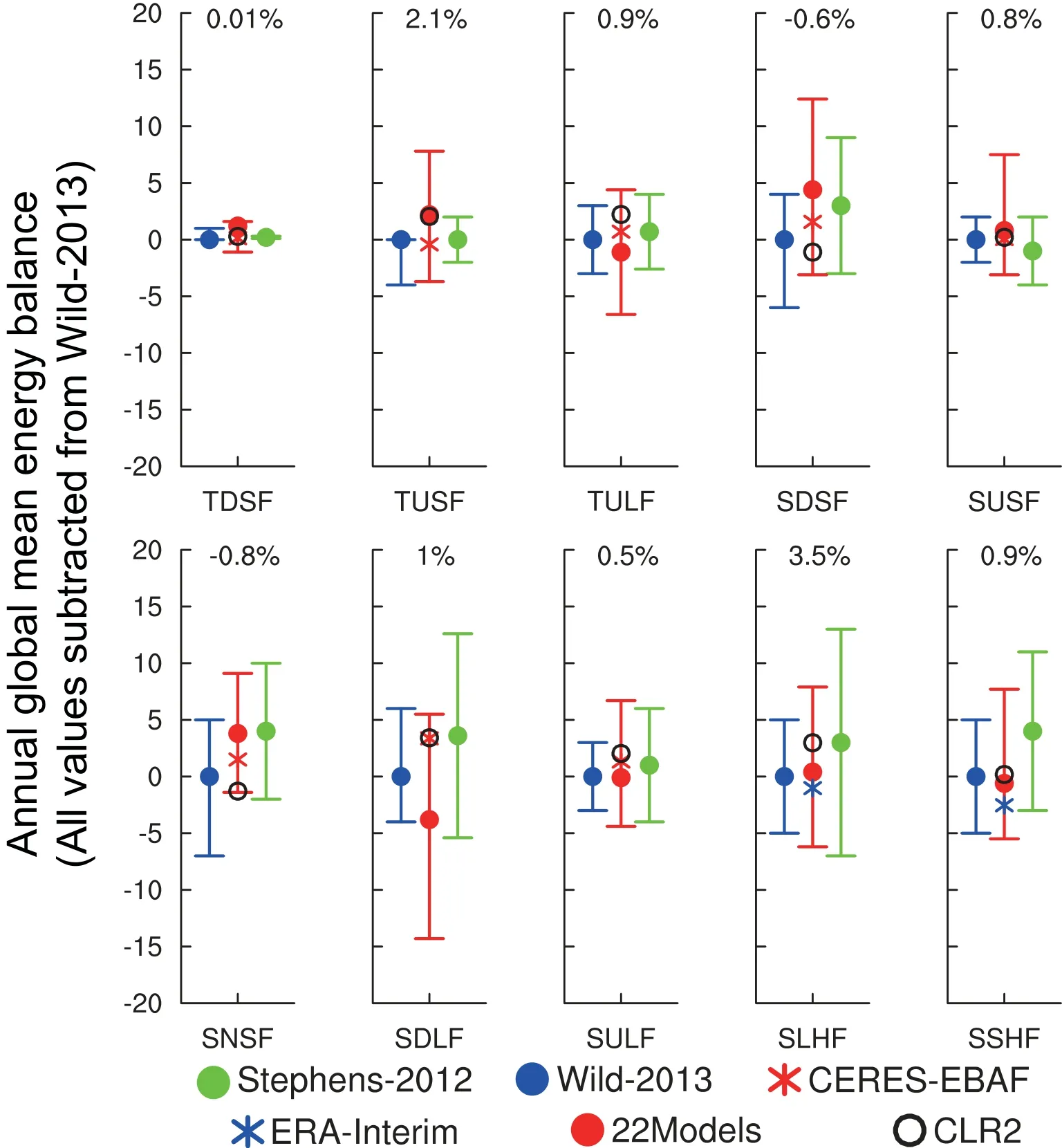
Fig.1.Annual global mean energy balance at the top of the atmosphere(TOA)and at the Earth’s surface in di f f erent datasets,including satellite products,reanalysis data,and the outputs from the 22 CMIP5 models.Units:W m−2.Those datasets parallel that of Zhou et al.(2015).The results have been subtracted from the values estimated in Wild et al.(2013).Green,blue and red error bars show the uncertainty ranges of two observational datasets,and the maximum and minimum values of the 22 CMIP5 models,respectively.The relative deviations[compared with Wild et al.(2013)]are listed at the top of echo subplot.The meaning of the abbreviations are as follows.TUSR—TOA upwelling shortwave radiation;TULR—TOA upwelling longwaveradiation;SDSR—surface downwelling shortwave radiation;SUSR—surface upwelling shortwave radiation;SNSR—surface net shortwave radiation;SDLR—surfacedownwelling longwaveradiation;SULR—surfaceupwelling longwaveradiation;SLHF—surface latent heat f lux;SSHF—surface sensible heat f lux.

4.2. Seasonal cycleof the global mean energy balance

To evaluatein moredepth theperformanceof FAMIL1.1 in simulating the energy balance,the seasonal cycle of the global mean energy balance was compared with CERESEBAF and ERA-Interim data(Fig.2).The CERES-EBAF satellite products were used to compare the radiative f luxes at the TOA and at the Earth’s surface,whereas the ERAInterim reanalysis data was used to compare the surface latent heat f luxesand surfacesensibleheatf luxes(SSHF)atthe Earth’ssurface.Theresultsshow that thesimulated seasonal cycle and amplitude of the radiation f luxes,as well as the surface heat f luxes,agree well with those from the observational/reanalysisdata.For example,the TOA upwellinglongwave radiation(TULR),the surface downwelling shortwave radiation(SDSR),and thesurfaceupwelling longwaveradiation(SULR),show strong seasonal cycles.They aregenerally stronger during thesummer and weaker during thewinter and have amplitudes of about 10,10,and 5 W m−2,respectively.FAMIL1.1 shows an equivalent change to these f luxes.The seasonal variations in the SLHF and the SSHF have weaker amplitudes(<3 W m−2)than the other variables in both the reanalysis datasets and the FAMIL1.1’s simulation.Thus,FAMIL1.1 simulates both the seasonal cycle and amplitude of theenergy balancereasonably well.

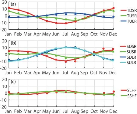
Fig.2.Seasonal cycle of global mean(a)TOA radiation f luxes,(b)surface radiation f luxes from CERESF-EBA(circles),and(c)surface sensible heat and latent heat f luxescalculated from ERA-Interim(circles)and FAMIL1.1(lines).The results have been subtracted from their global annual mean values.Units:W m−2.Abbreviations as in Fig.1.

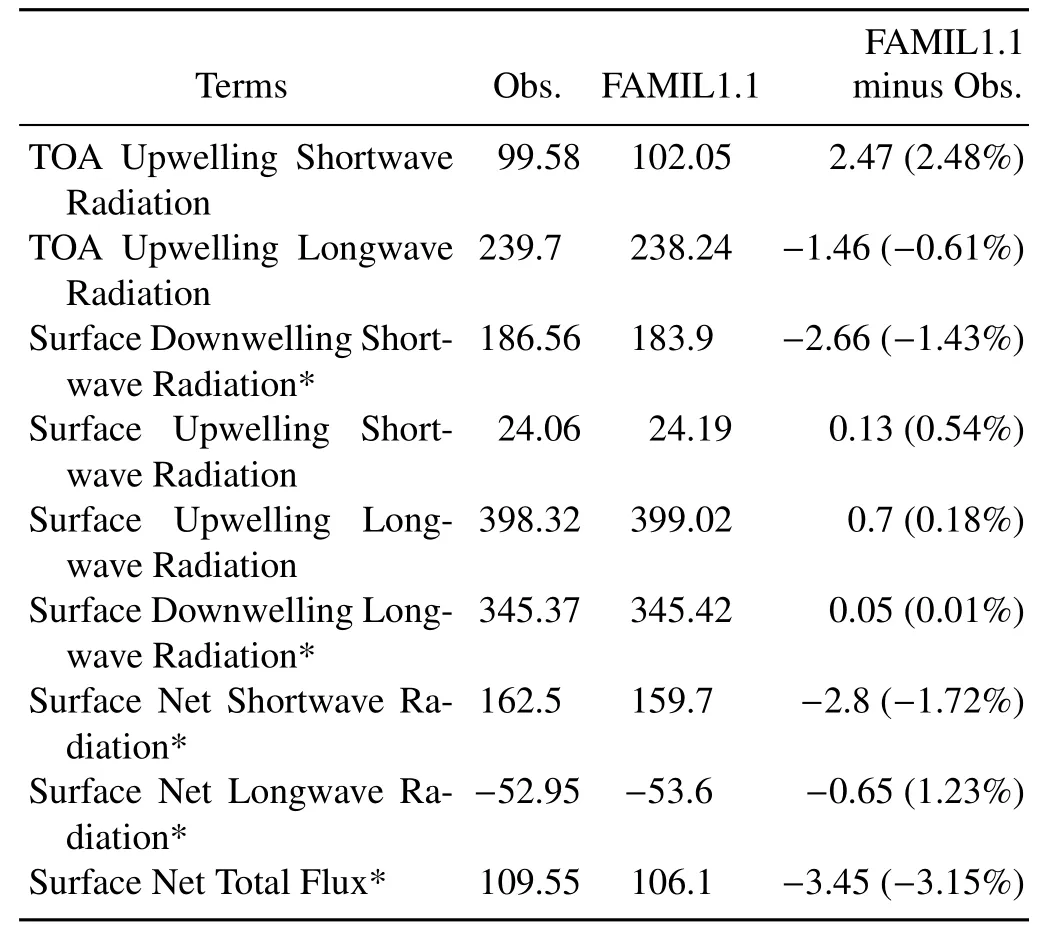
Table1.Comparisonsfor all-sky conditions.Hereafter,the*means positive downward.

4.3.Geographical distribution of theannual mean global energy balance

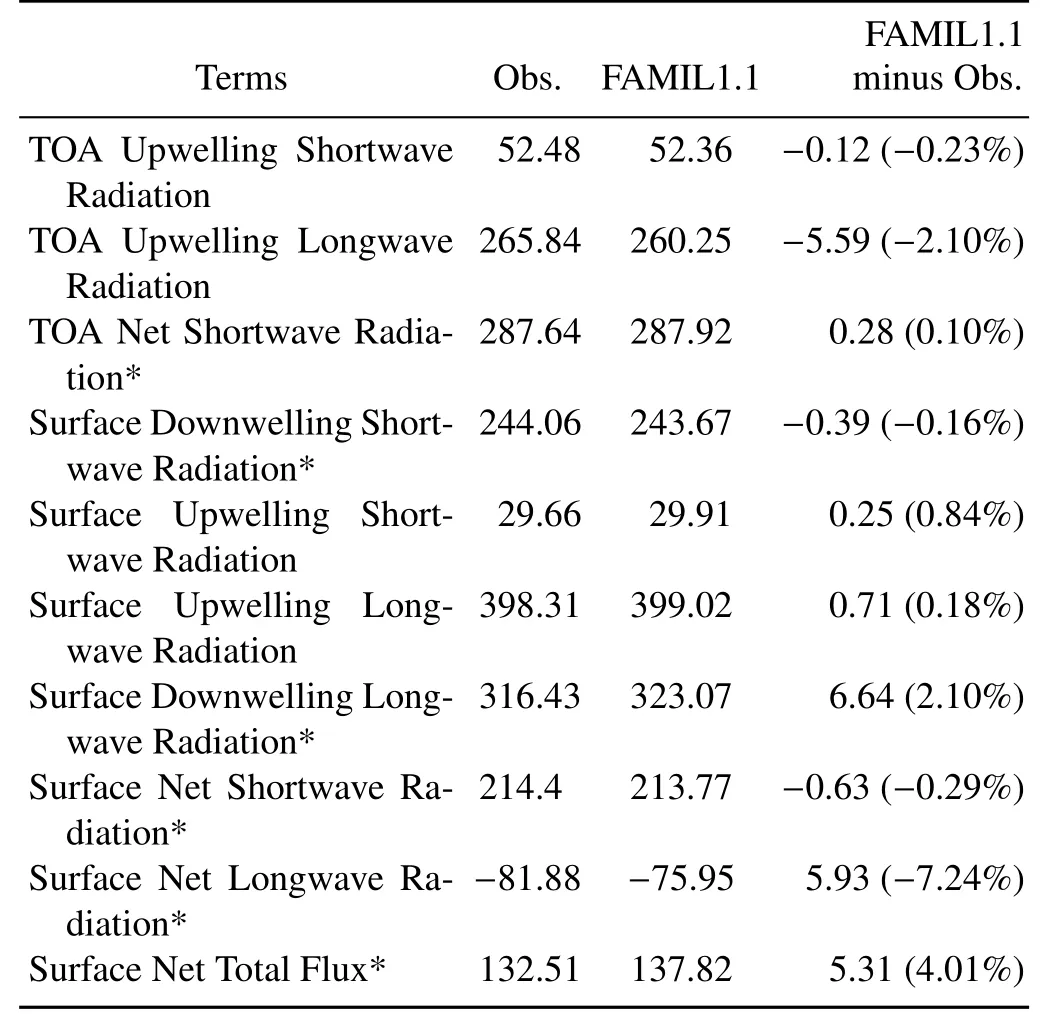
Table2.Comparisonsfor clear-sky conditions.

Global mean energy f luxes are of vital importance in characterizing the total energy balance in the atmosphere.However,global meansmay mask underlying regional di f f erences in energy balance.Thus,the geophysical distributions of various radiation f luxes are shown to further investigate the performance of FAMIL1.1 in simulating the global energy balance and regional biases.The most important term in the energy balance is the TOA net radiative f lux,which representsthetotal e f f ect of all thetermsconnected to theenergy balance.Thenet radiativef lux at the TOA isa f f ected by the TOA downwelling shortwaveradiation(TDSR),the TOA upwelling shortwave radiation(TUSR),and the TULR.The TUSR synthetically characterizes the total solar shortwave radiation ref lected by the earth system,including the comprehensiveref lection e f f ectsof clouds,surface/ocean albedo,and aerosols;et al.In contrast,the TULR represents the total outgoing longwave radiation emitted by the earth system,which isdetermined by thestructureof atmospheric temperature,theconcentration of greenhousegases,thetemperature/height of clouds,and theland/water emissivity,et al.

Figure 3 shows the annual mean geographical distribution of the TOA net radiation f luxes,the TUSR,and the TULR from the FAMIL1.1 and CERES-EBAF.Compared with CERES-EBAF,FAMIL1.1 reasonably reproduces the spatial distribution of the net radiative f luxes,as well as the TUSRand the TULR,withhighspatial correlationsof around 0.97,0.98,and 0.99,respectively.However,the RMSE is relatively large,at around 16.78,16.83,and 9.75 W m−2for the net radiative f lux,the TUSR and the TULR,respectively.Figure 3c shows that the main regional bias arises because the net radiative f lux over the most mainland areas in FAMIL1.1 is less than that observed(positive downward),with largenegativedeviationsin northern Africaand northern South America.The maximum negative deviation is about 60 Wm−2.Thenet radiativef lux over the Southern Ocean in FAMIL1.1 is also less than that observed(deviation of about−20 W m−2).By contrast,the tropical eastern Pacif ic Ocean isanareaof positivedeviations(maximumdeviation of about 50 W m−2).These biases are mainly aroused from the simulated biases in the geographical distribution of the TULR and TUSR.In northern Africa and northern South America,both the ref lected shortwave radiative f lux(maximum deviation of about 50 W m−2or 16%)and the upwelling longwaveradiativef lux(maximum deviation of nearly 10 Wm−2or 5%)are stronger than observed,which means that more of the radiative f lux is ref lected upward into space and contributesto thenegativedeviation in thenet radiativef lux.The deviationsin the Southern Ocean aremainly dueto astronger ref lected shortwave radiative f lux(deviation of about 20 W m−2or 18%).Over thetropical eastern Pacif ic Ocean,where persistent marine stratocumulus clouds are present,the ref lected shortwave cloud radiation is weaker than observed(maximum negative deviation of about 40 W m−2or 50%),whereas the outgoing longwave radiative f lux agrees well with theobservations,contributing to theoverall positivedeviation.Comparing Fig.3f and 3ialso showsthatdeviation in the net radiation f lux derives mainly from the simulated bias of the ref lected shortwave radiation over most of the regions,such as the Southern Ocean,northern Africa,northern South America,and thetropical eastern Pacif ic Ocean,in addition to the Atlantic Ocean.Theref lected shortwave radiation biases here should both result from the simulation bias for clouds and the ocean/land albedo,in addition to the aerosol’sdirect e f f ect.

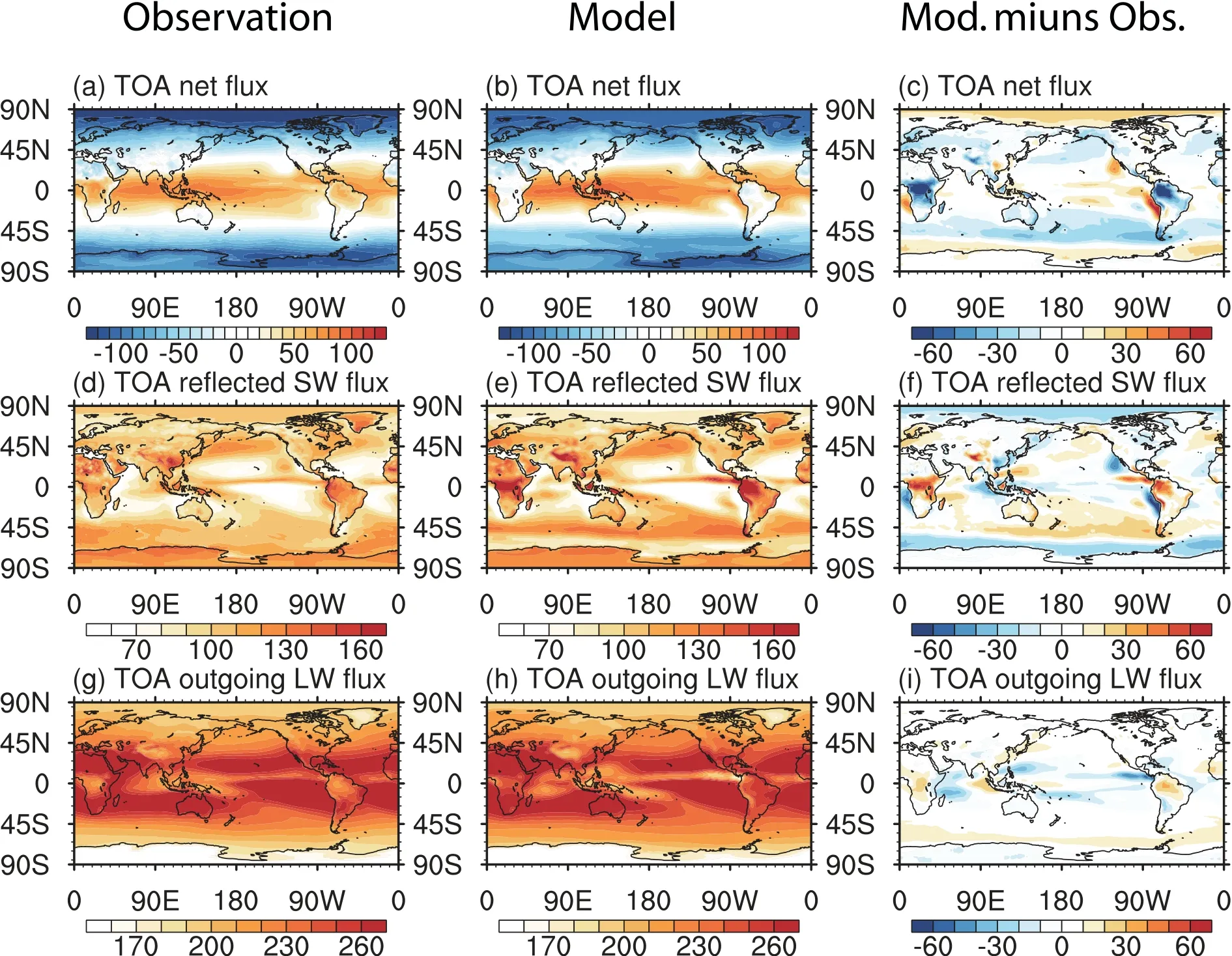
Fig.3.Geographic distribution of the TOA radiation f lux from FAMIL1.1 and observation(CERES-EBAF):(a–c)net radiation f luxes;(d–f)ref lected shortwave radiation f luxes;(g–i)outgoing longwave radiation f luxes.Units:W m−2.

Because the CLR2 mainly a f f ects the progress of cloud microphysics and therefore contributes to the CRF and energy balance of the Earth system,the ability of the model to simulate the CRF was further explored.Figure 4 shows the annual mean geographical distribution of the CRF in the atmosphere from the FAMIL1.1 and observations.FAMIL1.1 reproduces the spatial distribution of both the shortwave and longwave CRF reasonably well(spatial correlations of 0.96 and 0.93,respectively).However,the RMSEs for the shortwave and longwave CRF are 16.53 and 10.76 W m−2,respectively.Figure4f showsthatthemodel producesaweaker longwave CRFalmost everywhere,meaning thereisagreater outgoing longwave radiative f lux,as shown in Fig.3i.The shortwave radiative forcing is stronger in themodel than observed in northern Africa,northern South America,and the Southern Ocean,but weaker in the tropical eastern Pacif ic Ocean,thetropical eastern Indian Ocean,and the tropic eastern Atlantic Ocean.And the maximum deviation in these areas is almost 50 W m−2.These deviations are important contributorsto the biases in the TOA ref lected shortwave radiative f luxes.

Theoretically,the simulated bias in the cloud water content may have a good relationship with the deviation in the simulated shortwave cloud radiation,whereas the simulated bias in the amount of high clouds contributes to the simulated bias in the simulated longwave radiation forcing(Gettelman and Sherwood,2016).Figure5 showsthecloud water path(CWP)and amount of high clouds from the COSPsimulator and from observation(satellite retrievals).FAMIL1.1 reproduces the basic spatial distribution of the CWP in the CloudSat retrievals(Fig.5a and 5b),but with some regional biases.FAMIL1.1 tends to simulate a higher CWPover the oceans(including the tropical eastern Pacif ic Ocean,the Indian Ocean,and the Atlantic Ocean,except for the eastern oceans),and there is almost twice the amount of cloud water over theland(e.g.,South Americaand northern Africa)in the FAMIL1.1 than that in the satellite retrieval data.Figures 4 and 5 show that there is a good agreement for the simulation biases between the shortwave CRF and CWP.The shortwave CRF is stronger than the observed over the Southern Ocean,the northern Pacif ic Ocean,South America,and northern Africa,where the CWP is overestimated.By contrast,the CWP is underestimated over the eastern oceans,with a weaker shortwave CRF in FAMIL1.1.The model also reproduces a similar spatial distribution of the high clouds amount to the observational data,with a spatial correlation of around 0.94(Fig.5d and 5e).However,the high clouds amount is underestimated over South America,northern Africa,the Southern Ocean,and the northern Pacif ic Ocean,relative to the observations,with a maximum negative bias of 20%.The simulated bias for high clouds amount showsagood relationship with thesimulated biasfor the longwave CRF.For example,the amount of high cloud is underestimated over South America and northern Africa,with a weaker longwave CRFover theseregions.

4.4.East Asian energy balanceand e f f ectsof aerosols

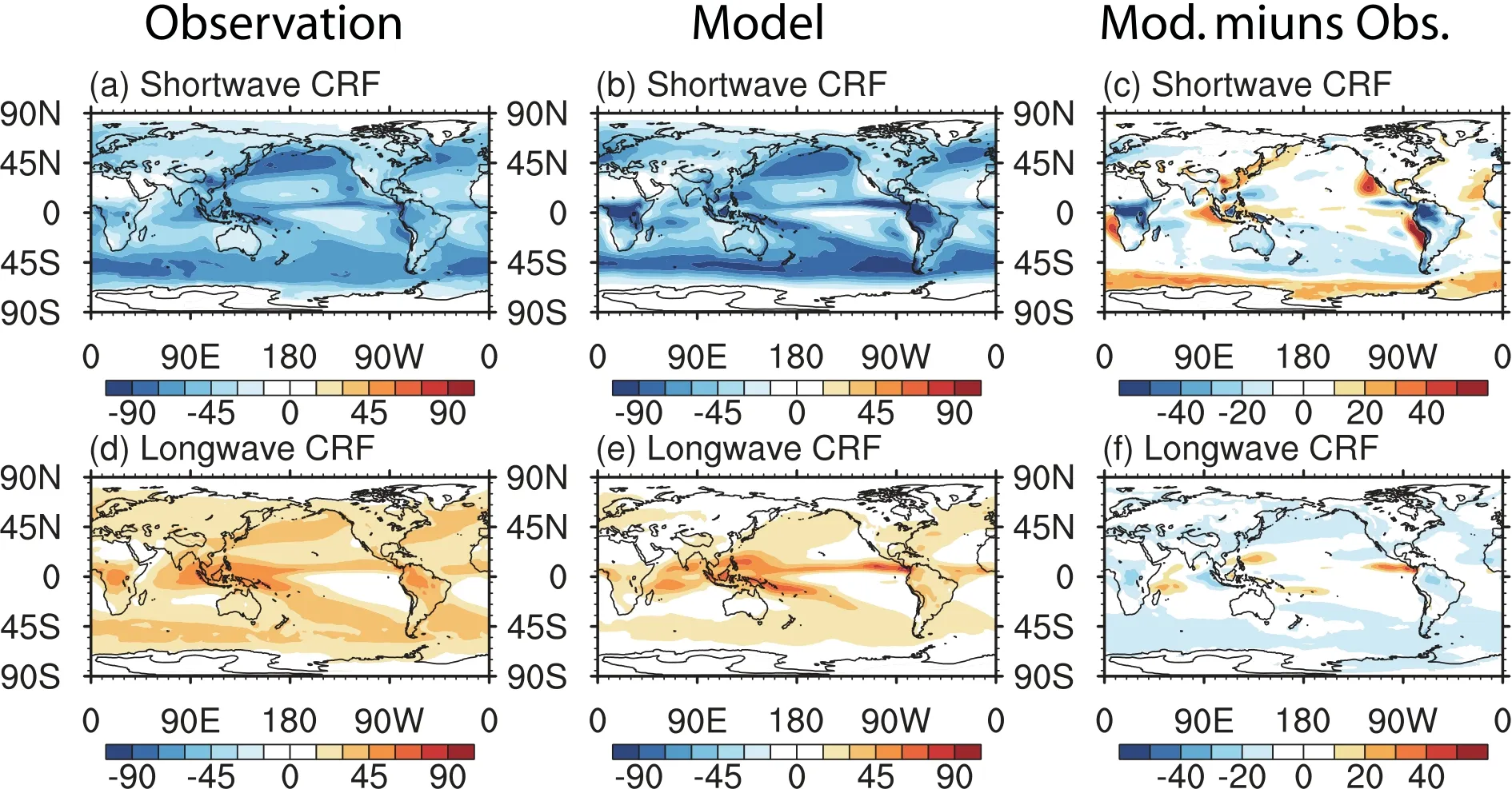
Fig.4.Geographic distribution of cloud radiation forcing from FAMIL1.1 and observation(CERES-EBAF):(a–c)shortwave cloud radiation forcing;(d–f)longwave cloud radiation forcing.Units:W m−2.

The AMR is an important climatic region with high observed concentrationsof aerosolsloading(Wang et al.,2012;Zhang et al.,2012).The distribution of the aerosol optical depth(AOD)at 0.55µm is a good representation of the distribution of the total aerosol loading.Figure 6 shows the geographical distribution of the total AOD at 0.55µm from the observation(MODIS)and FAMIL1.1.The model reproduces the distribution of AOD well,although it underestimates the AOD over East Asia(about 0.5 in FAMIL1.1,but>0.7 in the observational dataset).The underestimated AOD over East Asian mainly may result from thattheaerosol mass concentrations over East Asian are underestimated to some extent(Li et al.,2014a),which is also one of the important causes for the TOA radiation f luxes bias.Figure 7 shows the seasonal cycle of the shortwave and longwave CRF and the seasonal evolution of the CWP over the AMR(20◦–50◦N,70◦–130◦E).The model captures the seasonal evolution of the shortwave CRF and longwave CRF and the CWP reasonably well.For example,the anomalies in the shortwave CRFgradually increase from−13 W m−2in winter(December–January–February)to 40 W m−2in summer(June–July–August).FAMIL1.1 shows similar characteristics,with the anomalies varying from−16 W m−2to 45 W m−2.This means that the model gives an equivalent magnitude of shortwave CRF to the observations.However,the anomalies in the CWPvary from nearly−45 Wm−2in winter to 100 Wm−2in summer in theobservational dataset,but from−90 W m−2to 135 W m−2in the FAMIL1.1,which means that the model shows a much stronger variability for the CWP.

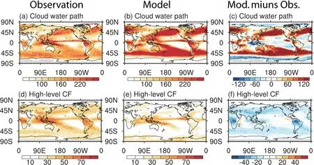
Fig.5.Geographic distribution of thecloud water path and amountof high level cloudsfrom observation(CloudSat/CALIPSO)and FAMIL1.1(with the COSPsimulator):(a–c)cloud water path(units:mg m−2);(d–f)high level cloudsfraction(CF)(units:%).

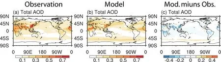
Fig.6.Geographical distribution of total aerosol optical depth(AOD)at 0.55µm from(a)observation(MODIS)and(b)FAMIL1.1.

Except for the seasonal cycle,previousstudies have also shown that there are seasonal di f f erences between summer and winter for the CRFover the AMR(Chen and Liu,2005;Lietal.,2017a).To further evaluatethemodel’sperformance in reproducing thisfeature,the geographic distribution of the CRF from FAMIL1.1 was compared with observations over the AMRduring summer and winter time(Fig.8 and Fig.9).Observationally,the main feature of the CRF in summer is thattherearelarger shortwave CRFover the AMR,especially over the southeastern Tibetan Plateau,eastern China,and the East China Sea(Fig.8a).The average shortwave CRF over the AMR is−69 W m−2.The longwave CRF is larger over the Bay of Bengal and eastern China(Fig.8d),witharegional mean about 40 W m−2over the whole AMR.FAMIL1.1 reproducesthegeographical distribution of the shortwave CRF and longwave CRFin summer well,with an averaged shortwave CRF about−71 W m−2and an averaged longwave CRFabout 28 Wm−2.However,FAMIL1.1 showsastronger shortwave CRF over the Tibetan Plateau,but weaker over eastern Chinaand the East China Sea.FAMIL1.1 also underestimatesthelongwave CRFover thewhole AMR.Theaverage negative deviation is about 12 W m−2(or 30%).Figure 9a and 9d also show that the shortwave CRF and longwave CRF decreased greatly over the whole AMR from summer to winter.The averaged shortwave CRF and longwave CRF over the AMR are about−24 and 16 W m−2,respectively.In observation,there is a larger shortwave CRFover eastern China and the East China Sea(>60 W m−2),but a weaker shortwave CRF over the Tibetan Plateau and its surrounding areas(<30 Wm−2).FAMIL1.1 reproducesthe summer–winter contrast for both the shortwave CRF and longwave CRF,but their magnitudes are biased.The averaged shortwave CRF and the longwave CRF over the AMR are about−14 and 5 W m−2,respectively,which means that the average biases are 10 W m−2(40%)and 11 W m−2(66%)over the AMR,respectively.By contrast,FAMIL1.1 seems to underestimate the shortwave CRF over eastern China and the Tibetan Plateau and showsa weaker longwave CRFover the whole AMR.

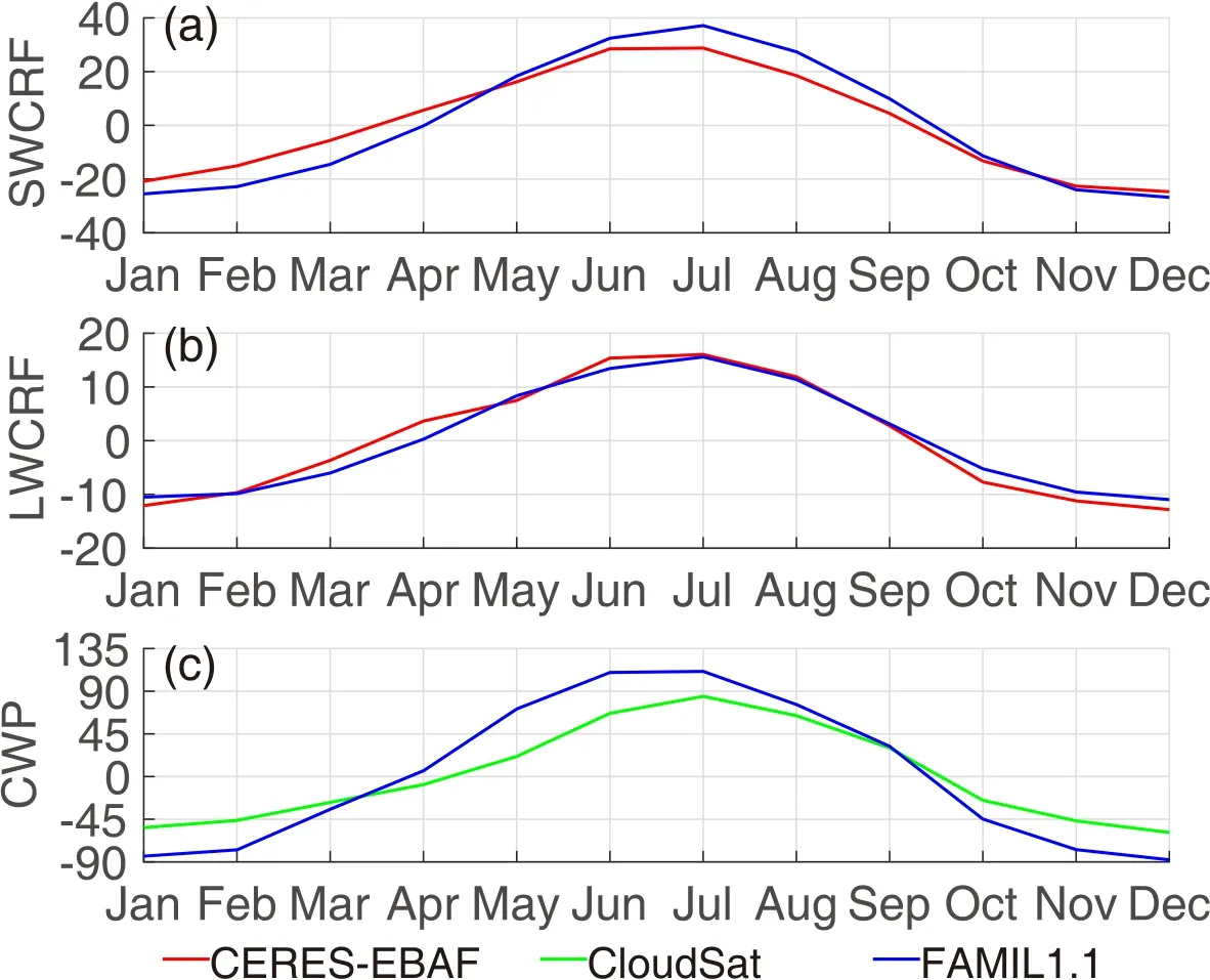
Fig.7.Seasonal cycle of cloud radiation forcing(units:W m−2)and cloud water path(units:mg m−2)from FAMIL1.1 and observation(CERESEBAF/CloudSat)in the AMR(20◦–50◦N,70◦–130◦E):(a)shortwave cloud radiation forcing(SWCRF);(b)longwave cloud radiation forcing(LWCRF);(c)cloud water path(CWP).Axesintervals have been subtracted from their annual mean values.

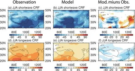
Fig.8.Geographic distribution of cloud radiation forcing from FAMIL1.1 and observation(CERES-EBAF)over the AMR(20◦–50◦N,70◦–130◦E)in summer(June–July–August):(a–c)shortwave cloud radiation forcing;(d–f)longwave cloud radiation forcing.Units:W m−2.

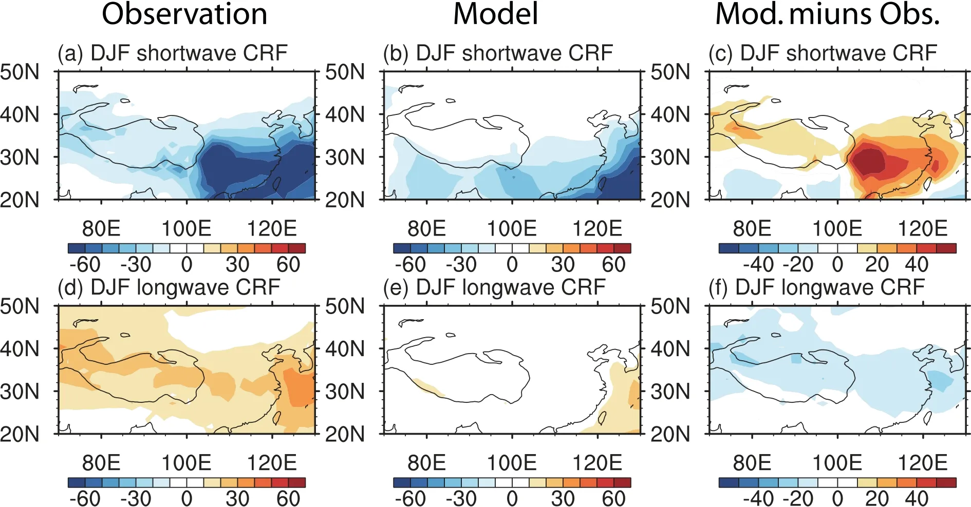
Fig.9.Geographic distribution of cloud radiation forcing from FAMIL1.1 and observation(CERES-EBAF)over the AMR(20◦–50◦N,70◦–130◦E)in winter(December–January–February):(a–c)shortwave cloud radiation forcing;(d–f)longwave cloud radiation forcing.Units:W m−2.

In theory,the cloud water mass concentration and the cloud droplet radius will both change the shortwave CRF.Smaller cloud droplets usually lead to clouds with a higher albedo(Peng et al.,2002)and thusthe ref lection of moresolar radiation.Figure 10 shows the scatter plots of the seasonal mean shortwave CRF versus the CWP over continental East Asia(20◦–40◦N,100◦–120◦E)and the northern Pacif ic Ocean(20◦–40◦N,170◦E–170◦W).Comparisonof these two areas(land and ocean)highlights the importance of the droplet radiusin shortwave CRF.And aerosol conditionsdifference may be one of the reasons for the land-seadi f f erence because of its vital importance on the cloud activation process,which can be physically described by CLR2 scheme.Observationally,the slope of these plots over land is larger than over the ocean(slope of 0.29 versus 0.1).One of the possible reasons for the slope di f f erence may be attributed to thedi f f erence of theaerosol background over land and ocean area.The land is often much polluted than the ocean,which provides a high concentration of CCNs.As the amount of cloud water increases,more abundant and smaller droplets are produced over the land than over the ocean,resulting in a stronger CRF(greater slope).This relationship can also be reproduced in FAMIL1.1,but the di f f erencesbetween the ocean and land arelesssignif icant(slopeof 0.21 versus0.08)than observed.Thereason may bethat aerosol massconcentration over East Asian used in thisstudy islargely underestimated than observed(Lietal.,2014a),whilecomparableover oceans to some degree in FAMIL1.1.This is also seen in the distribution of the AOD.In general,the model can simulate thecontrastbetween theland and oceansin termsof theassociation between the cloud water content and shortwave CRF,but this association is weaker over East Asia in FAMIL1.1 than observed.

5.Discussionsand conclusions

This study describes the incorporation of a twomoment(massand number)cloud microphysicsschemeinto FAMIL1.1 with theaim to simulatecloud microphysical processes more realistically,including the subgrid-scale updraft velocity for cloud droplet activation.The global and regional characteristics of the energy balance and CRF simulated by FAMIL1.1 wasevaluated using a comprehensive suite of observational and reanalysisdata.

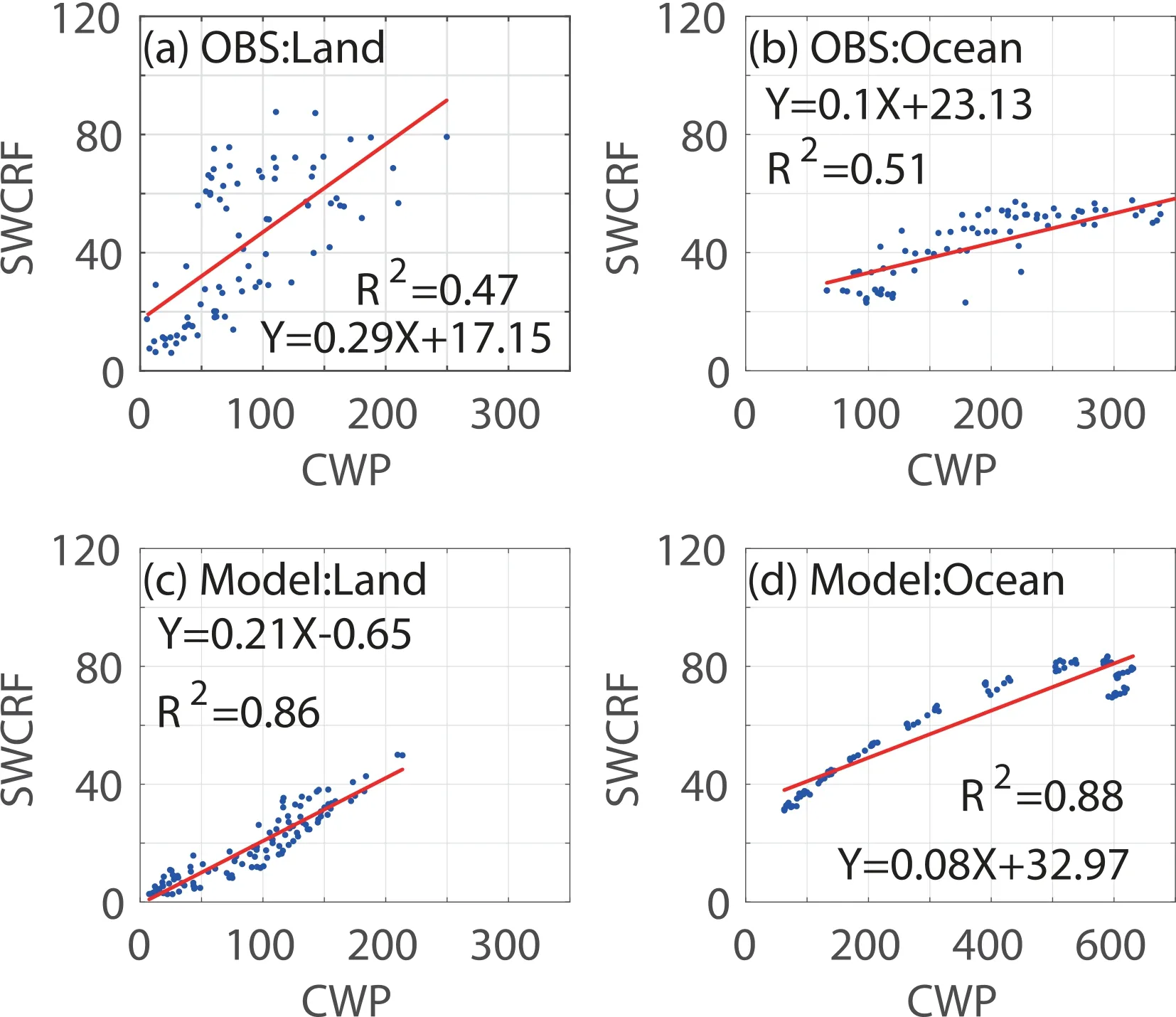
Fig.10.Scatterplots of the(a,b)observed and(c,d)modeled(FAMIL1.1)seasonal mean shortwave cloud radiation forcing(SWCRF)versuscloud water path(CWP)over(a,c)continental East Asia(20◦–40◦N,100◦–120◦E)and(b,d)the northern Pacif ic Ocean(20◦–40◦N,170◦E–170◦W).

The global annual means of the simulated radiative/heat f luxes in FAMIL1.1,both at the TOA and at the Earth’s surface,generally agree well with the observational/reanalysis data.FAMIL1.1 also simulateswell in theseasonal cycleand amplitudeof theradiation and surfaceheat f luxes,suggesting that the CLR2 scheme has been successfully introduced into FAMIL1.1.

Also studied was the geographic distribution of the TOA radiative f lux and CRF,revealing that FAMIL1.1 reproduces thegeographic distribution of theradiation f luxeswith ahigh spatial correlation to observations.The main regional biasis that the net radiative f lux over the mainland in FAMIL1.1 is less than that in the observational data,with large negative deviations in northern Africa and northern South America.By contrast,theeasternoceans(marinestratocumulusregion)show positive deviations,in good correspondence with the CRF.Further analysis shows that the deviations of the CRF can bepartly ascribed to thesimulated deviationsof the CWP and the amount of high cloud.The model is also able to reproduce the seasonal evolution of the CRF and CWP over East Asia.Furthermore,it reproduces the summer–winter contrast for the geographic distribution of both the longwave CRF and shortwave CRF over the AMR,and simulates the contrast between theland and oceansin termsof theassociation between thecloud water content and shortwave CRF.

In conclusion,FAMIL1.1 performswell in thesimulating of the global energy balance as well as the regional features over the AMR,asverif ied by investigatingitsspatial and temporal features.However,there is a large simulation bias in terms of CWP and the amount of high cloud over both the land and ocean,concentrating the simulated deviationsin the radiative f lux.The reasons for these simulation biases will be investigated in future work based on the large-scale atmospheric circulation,precipitation,and other detailed outputs from the COSPsimulator.The present study uses a uniform assumption to derivethevertical velocity in the PBL scheme to determine the change of saturation.The uncertainty in PBL schemeaswell asthesub-grid-scalevelocity should also betested in futurework.Currently,theaerosol concentration in FAMIL1.1 is prescribed,but work is now taking place on an aerosol module that determines the aerosol concentration dynamically.Theimpactof thehorizontal resolution and air–sea coupling processes on the performance of the model also needsto bestudied further.

APPENDIX

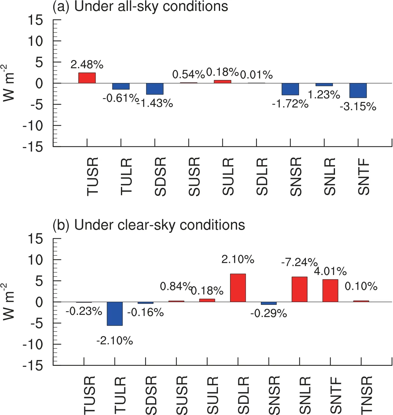
Fig.A1.Annual global mean energy balancebias(FAMIL1.1 minus CERES-EBAF)at the top of the atmosphere(TOA)and at the Earth’s surface under(a)all-sky conditions and(b)clear-sky conditions.Units:W m−2.The relative deviations are listed at thetop of each bar.The meaning of the abbreviations isthe sameasthat in Fig.1.,in addition to:SNLR—surface net longwave radiation;SNTF—Surface Net Total Flux;TNSR—TOA Net Shortwave Radiation.This f igure is an illustration in parentheses with Table 1 and Table2.

Acknowledgements.We thank two anonymous reviewers for their careful reading of the manuscript and their many insightful comments and suggestions.This study was jointly funded by the National Natural Science Foundation of China(Grants 41675100,91737306,and U1811464).