Simulation and prediction of monthly accumulated runoff,based on several neural network models under poor data availability

JianPing Qian , JianPing Zhao , Yi Liu , XinLong Feng , DongWei Gui *

1. College of Mathematics and System Sciences, Xinjiang University, Urumqi, Xinjiang 830046, China

2. State Key Laboratory of Desert and Oasis Ecology, Xinjiang Institute of Ecology and Geography, Chinese Academy of Sciences, Xinjiang 830011, China

3. Cele National Station of Observation and Research for Desert-Grassland Ecosystem, Xinjiang Institute of Ecology and Geography, Chinese Academy of Sciences, Urumqi, Xinjiang 830011, China

ABSTRACT Most previous research on areas with abundant rainfall shows that simulations using rainfall-runoff modes have a very high prediction accuracy and applicability when using a back-propagation (BP), feed-forward, multilayer perceptron artificial neural network (ANN). However, in runoff areas with relatively low rainfall or a dry climate, more studies are needed. In these areas—of which oasis-plain areas are a particularly good example—the existence and development of runoff depends largely on that which is generated from alpine regions. Quantitative analysis of the uncertainty of runoff simulation under climate change is the key to improving the utilization and management of water resources in arid areas. Therefore, in this context, three kinds of BP feed-forward, three-layer ANNs with similar structure were chosen as models in this paper.Taking the oasis-plain region traverse by the Qira River Basin in Xinjiang, China, as the research area, the monthly accumulated runoff of the Qira River in the next month was simulated and predicted. The results showed that the training precision of a compact wavelet neural network is low; but from the forecasting results, it could be concluded that the training algorithm can better reflect the whole law of samples. The traditional artificial neural network (TANN) model and radial basis-function neural network (RBFNN) model showed higher accuracy in the training and prediction stage. However, the TANN model, more sensitive to the selection of input variables, requires a large number of numerical simulations to determine the appropriate input variables and the number of hidden-layer neurons. Hence, The RBFNN model is more suitable for the study of such problems. And it can be extended to other similar research arid-oasis areas on the southern edge of the Kunlun Mountains and provides a reference for sustainable water-resource management of arid-oasis areas.

Keywords: oasis; artificial neural network; radial basis function; wavelet function; runoff simulation

1 Introduction

The effective use of water resources is critical to the sustained development of society and the economy, especially in semiarid and arid areas where their fragile environment and ecosystems are seriously threatened by water scarcity and irrational exploitation (Boehmer et al., 2000; Chapman and Thornes, 2003; Skirvin et al., 2003; Meng et al.,2009). Xinjiang, located in the northwestern part of China, is the largest and most widely distributed area of arid-oasis landscape in China. Its dense population,fragile ecological environment, and water scarcity all threaten the sustainable development of the oasis area in Xinjiang (Chen et al., 2009; Wu et al., 2010; Li et al., 2011a,b). Water resources, the most crucial factor for the development of these oases, basically rely on the mountain runoff originating from the Kunlun Mountains. Accurately estimating and predicting river flows is critical both for short-term and long-term risk assessment of river basins, as well as for water-resources management and planning decisions (Ling et al., 2011; Chen, 2014). Runoff, like other natural processes, is determined by a variety of independent variables involving different dynamics and nonlinear physical mechanisms or systems. After years of development, a variety of methods has been developed to predict river runoff, such as linear and nonlinear time-series methods, gray system theory, physical models, conceptual models, artificial neural network(ANN) models, or mixed models integrating two or more of these approaches (Zhang and Govindaraju,2000; Nourani et al., 2009a; Sun et al., 2016).

In recent years, ANNs have been widely used in ecological and hydrological research and successfully applied to the simulation and prediction of river runoff (Wu et al., 2009). As ANNs have been applied and developed over a long period, many improvements and deformation forms of ANNs come to the fore. ANNs have shown considerable ability in modeling and forecasting nonlinear hydrological timeseries and solving complex problems; notwithstanding, they are always black-box in type, using a datadriven approach and a function approximator (Kisi and Cigizoglu, 2007; Nourani et al., 2009a). Traditional ANN (TANN) models have good nonlinearity and self-learning ability, which can solve the problems of hydrological forecasting and achieving good simulations (Jain et al., 1999; Salas et al., 2000; Campolo et al., 2003; Hu et al., 2005; Nilsson et al.,2006). Nonetheless, such models have many shortcomings, such as their susceptibility to oscillation,slow convergence, falling toward the local minimum,and difficulty in determining the number of hiddenlayer neurons. To overcome these problems, the compact wavelet neural network (CWNN) was developed(Licznar and Nearing, 2003; Adamowski and Chan,2011; Ramanik et al., 2011). The structure and expression of a CWNN are basically the same as in a TANN—that is, comprising three layers: the input layer, hidden layer, and output layer. The main difference lies in that a CWNN uses the wavelet function as the activation function. The characteristics of the wavelet function allow the CWNN to achieve a better-fitting effect when dealing with the variables of random vibration and periodic changes (Kim et al.,2006; Partal and KişI, 2007; Nourani et al., 2009b).Another improved neural network approach is the radial basis-function neural network (RBFNN), which is a three-layer, static feed-forward neural network in structure. The number of hidden-layer units and the structure of the network are adjusted adaptively during the training phase, according to the specific problems being studied. Therefore, this network approach offers improved applicability. Neural network models do not require hydrological characteristics when being applied to water-management issues; rather, one simply needs to select the appropriate model and network structure (Bowden et al., 2005a,b). However,the high degree of nonlinearity and instability of the runoff time-series, coupled with the abnormal changes of river runoff caused by climate change in recent years, has introduced more uncertainties into the simulations by neural networks applied in this field.

The Qira River Basin, a typical inland river watershed on the southern rim of the Tarim Basin, is characterized by a mountain-oasis-desert ecosystem, owing to its different climatic characteristics (Wu et al.,2011, 2013). In recent years, oasis areas in the Qira River Basin have had to be opened up due to the rapid increase in population and the pressure of maintaining economic growth. The immediate consequence is overexploitation of Qira's water resources, resulting in a gradual reduction of water availability and multiple dry-out episodes in the lower reaches of the river(Ninyerola et al., 2000; Jeffrey et al., 2001; Xue et al., 2017a,b). Due to the lack of short-term and medium-term early warning systems for runoff, floods frequently occur in the middle and lower reaches of the Qira River during the flood season, posing a substantial threat to the lives and property of residents along the river bank.

Previous studies have shown that neural network models can be highly accurate and achieve a good fitting effect when applied to the prediction of the area of runoff, with rainfall as the main driving force.Therefore, in this study, we selected three kinds of three-layer, feed-forward neural network models(TANN, CWNN, and RBFNN) with similar structures; and we simulated and forecasted the runoff of the Qira River. There are two important issues in the network construction and learning process. The first is the lack of available meteorological and hydrological data in the region of the upper Qira River (Fang et al.,2011); and second, the flow of rivers in previous studies were less affected by seasonal changes, so the monthly runoff did not change significantly from year to year. However, the Qira River has a flood season and dry periods, meaning the annual runoff varies greatly (Xue et al., 2015, 2016). These two points make the neural network more sensitive to the selection of input variables when one is carrying out simulations and predictions in the Qira River Basin. Fortunately, previous research results and the applicability of the model have solved this problem. By using existing meteorological and hydrological data and an ap-propriate neural network model, accurate simulation and prediction of Qira River runoff is sufficient to provide a decision-making basis for water use and disaster prevention on both sides of the riverbank (Dai et al., 2009a,b).

2 Materials and methods

2.1 Study area and data

The Qira River Basin is located in the middle of the northern foot of the Kunlun Mountains in Xinjiang, China (36°02′N-37°16′N, 80°07′E-81°00′E),with a coverage area of about 3,328.51 km2(Figure 1).The Qira River is about 136.2 km long and originates in the high-altitude valleys of the Kunlun Mountains,flowing through the plain-oasis landscape and eventually disappearing at the southern edge of the Taklamakan Desert (Dai et al., 2009a,b). The southern margin of the Tarim Basin, in which the Qira River Basin is located, is dotted with a large number of oases. The freshwater recharge for each oasis is dependent on the surface runoff formed by the high valleys of the Kunlun Mountains, where the surface runoff is shaped by the melting of glaciers, snow, or the occurrence of rainfall. The precipitation in alpine areas occurs mainly as snowfall and is temporarily stored in the snowpack and/or ice caps, whereas precipitation over oases and deserts cannot form effective water (Wu et al., 2011, 2013).

The availability of meteorological data in this basin area is very poor. There is only one long-term weather station in Qira County, located in the downstream area of the river (1,337 m a.s.l.). A hydrological station (1,557 m a.s.l.) is available at a distance of 27 km from the mountain area. The station was established to provide long-term runoff data, but there is no long-term meteorological or hydrological station in the Kunlun Mountains at the source of the Qira River.However, these missing meteorological data are important data affecting the Qira River's runoff. Therefore, this study could rely on only a meteorological and hydrological dataset—including monthly mean temperature (MMT), monthly accumulated precipitation (MAP), monthly accumulated evaporation(MAE), and monthly accumulated runoff (MAR)from 1981 to 2008, obtained from the middle and lower reaches of the Qira River; and then use the neural network models to predict the MAR of the Qira River one month in advance. The uncertainty and accuracy of the model will be affected by data availability; the selection of input variables and the number of hidden nodes have a substantial impact on the model output.

The runoff, temperature, precipitation, and evaporation time-series are illustrated below. Seventy percent of the data from the beginning of the study period were used for model-learning, and the remaining 30% were used for the testing and prediction of model performance. Before using these data, we needed to remove any abnormal values and outliers via interpolation, which can improve the reliability and authenticity of the data (Dawson and Wilby, 2001; Wang et al., 2006). To map the data linearly between -1 and 1,the mathematical expression is

where, for each time-series, xiis the n ormalized value,xiis the observed time-series,and xminandxmaxare minimum and maximum values of theobserved values, respectively.

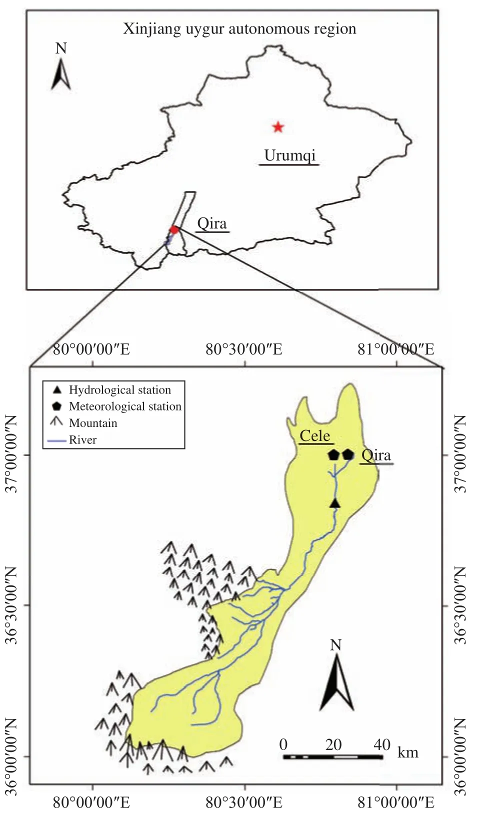
Figure 1 Location and topography of the study area

The neural network model has a great dependence on the training samples. Therefore, Step 1: This paper analyzes the statistical characteristics of the hydrological time-series variables used in the paper and selects the appropriate neural network model to simulate the samples. Step 2: Normalize all time-series variables in the text. Step 3: The neural network input variables are compared horizontally to the performance of the three types of neural network models. Step 4: Select the appropriate input variables and the number of hidden-layer neurons, to get the optimal model structure and optimal analog output. Step 5: Analyze the reasons for the difference in accuracy of the three types of network models in the hydrological prediction of the Qira River Basin and determine the optimal model and model structure for hydrological prediction in this area.

2.2 TANN

A TANN is defined as a structure consisting of a series of simple, interconnected operating elements known as neurons (units, cells, or nodes in the literature), inspired by biological nervous systems. The network can perform special-function mappings between inputs and outputs by adjusting the connection(weights) between neurons. The important decisions that need to be made when establishing the neural network model include selecting the neural network type,the network structure, the training algorithm, the input/output data-preprocessing method, and the training-stop criterion (Nourani et al., 2009a). The establishing the neural network model provides a general framework for representing a set of nonlinear function mappings between input and output variables.Hence, TANNs have attracted considerable attention in the past few decades and have been widely used in estimating and forecasting hydrology, climate, and other variables.

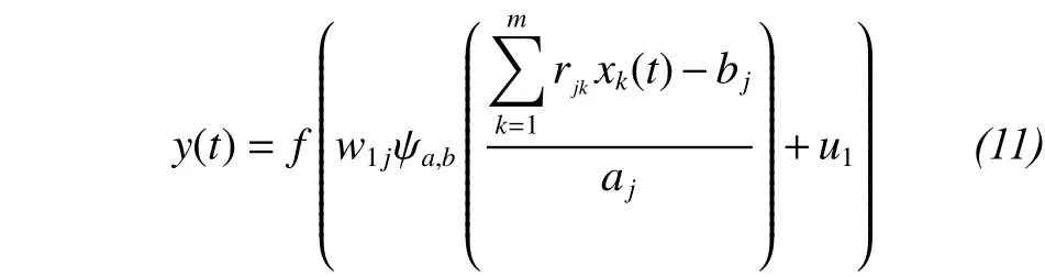
In previous research, the feed-forward multilayer(FFML) ANN models based on BP learning algorithms have been the most popular type. In particular, a three-layered nonlinear neural network can give an arbitrary approximation of a continuous function with any precision (Figure 2). We used BP learning algorithms in the present study because they have been the most widely used ANNs for hydrological models and applied to water-resources problems in recent years (Srinivasulu and Jain, 2006). The first and last layers are called the input and output layers, and the other layers are all hidden. The network includes several connected neurons, together called a typical FFML network. The most basic task of establishing a network is to determine the number of hidden layers and neurons (i.e., the network structure). It is still common to use trial-and-error methods to determine the number of network nodes at different layers (Cannas et al., 2006). The output value of the TANN can be expressed as follows:

In this formula, m and n are the number of input and hidden neurons, respectively (I= 1, 2, 3, ..., m and j =1, 2, 3, ..., n). wj0and ok0are the deviations of the jth neurons of the hidden layer and the kth neurons of the output layer, respectively; wjiand okjare the connection weights between the ith neurons of the input layer and the jth neurons of the hidden layer and between the jth neurons of the hidden layer and the kth neurons of the output layer, respectively; xirepresents the ith input variable of the input layer; ykrepresents the output value of the kth output of the output layer; and f0and fhare the activation functions of the output neuron and the hidden neuron,respectively. The activation functions commonly used in TANN are linear and tan-sigmoid functions, and their general equations are as follows:

where c ＞0 is a positive-scaling constant, and x is from a range of [-∞, +∞].

Figure 2 Schematic diagram of a three-layered ANN

2.3 RBFNN

Moody and Darken (1988) first proposed the RBFNN; and then, in the next few years, the uniform approximation performance of the radial basis-function network was demonstrated for nonlinear continuous functions. Thus far, several RBF network-training algorithms have been proposed. The excellent characteristics of the RBFNN make it another neural network type with the potential to replace BP networks;and it has therefore been widely used in various fields. As with BP networks, RBFNNs are static forward networks. Their topology is as follows: in an RBFNN with three layers, the first layer is the signalinput layer, the second layer is the nonlinear transformation layer, and the third layer is the linear convergence layer, i.e., the output layer of the network.The output of the nonlinear transform layer is:

where x=[x1, x2, ..., xn]Tis the input vector, ci= [c1i,c2i, ..., cni]Tis the central vector of the ith nonlinear transformation unit, I= 1, 2, ..., M, in which M is the output dimension;is the width of the ith nonlinear transformation unit; ||*|| is 2-norm; and g(*) denotes a nonlinear function, which is generally regarded as a Gaussian function:

The function of the linear merge layer is to combine the output linear weights of the transform layers. The output is

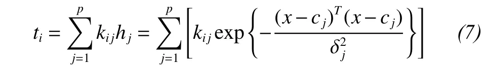
where I= 1, 2, ..., M, in which M is the output dimension; p is the number of hidden-layer elements,andis the weight of the jth neurons of the hidden layer to the ith neurons of the output layer.

2.4 CWNN

A CWNN is a new neural network model constructed by combining wavelet-transform theory and the ANN approach. It consists of an input layer, hidden layer, and output layer. The method replaces the traditional activation function of the neurons in the hidden layer of the neural network with the wavelet function, while the corresponding weights and thresholds are replaced by the scale and translation parameters of the wavelet basis function. As such, it fully inherits both the good time-frequency localization of the wavelet transform and the advantages of the neural network self-learning function, thus possessing the characteristics of strong fault tolerance,faster convergence speed, and improved forecasting(Mallat, 1998; Labat et al., 2000).

At present, spline wavelet and Morlet wavelet have good local smoothness. The scaling and translation factors of these functions can constitute the standard orthogonal basis of L2(R), so that the resulting wavelet series can best approximate the objective function. In this paper, the Morlet wavelet function is used in the hidden layer. The expression is

The wavelet transform for the square integrable Hilbert space o f L2(R), if there is a function,, and the Fourier transform satisfies the following form:

where: a, b ∈ R, a ≠ 0, in which a and b are scale and translated scale factors, respectively.

In this paper, the CWNN has three layers, and the number of neurons in the three layer is n, m, and 1, respectively.is the activation function of each hidden-layer neuron, and the output-layer neuroactivation function is sigmoid, meaning the output expression is

2.5 BP algorithm

To ensure the performance of the ANN model, it is necessary to adjust some parameters, such as the number of iterations, the number of neurons in the hidden layer, the weight, and the deviation, accordingly. These steps are usually implemented through ANN training. You can use different types of algorithms to train ANNs, including gradient descent and faster operations using heuristics or optimization algorithms (Beale and Demuth, 1998; Chen et al.,2015). In this work, the BP algorithm was used to train the neural network model. This algorithm is usually faster and easier to apply than other training methods.

The basic idea of the BP algorithm is that the learning process consists of two parts: the forward propagation of the signal and the reverse propagation of the error. In the forward propagation, the input samples are passed from the input layer and pro-cessed by the hidden layers to the output layer. If the actual output of the output layer does not meet the required output accuracy, then the error of the reversepropagation phase begins (Hagan and Menhaj, 1994;Ham and Kostanic, 2000). Error back propagation is the output error in some form through the hidden layer to the input layer by layer reverse propagation, and the error is distributed to all layers of the unit, so as to obtain the error signal of each layer unit. The weightadjustment process is the network-learning and -training process. This process continues until the network output error is reduced to an acceptable level or to a preset number of learning times. The mathematical expression of the BP algorithm is

where w is the weight, threshold, or parameter that needs to be corrected; ƞ is the preset network-learning rate; ykis the observed value of the kth training sample; and tkis the network-output value of the kth training sample.

2.6 Performance-evaluation criteria

The statistical error measurements used in this study to assess the performance of the different models are the coefficient of determination (R2), Nash-Sutcliffe efficiency (NSE), and percentage bias (PBIAS). All these indicators are used as a statistical indicator to evaluate the verification and calibration performance. Their expressions are as follows:

The R2statistic shows the degree of fitting between the observed and predicted data. The value range of R2is [0, 1], where an R2value closer to 1 indicates a better degree of fitting between the regression line and the observed value; and a value closer to 0 indicates consistency between the observed and estimated values. The theoretical value of NSE is between -∞ and 1, and NSE uses the value greater than zero as an indicator to evaluate the consistency between the observed and estimated values. If the value of NSE is close to 1, it indicates that the estimated data series is close to the observed value (Moriasi et al., 2007). The PBIAS can measure the model outputs that are less than or greater than the corresponding observations and provides a clear indication of the performance of the model (Gupta et al., 1999;Li et al., 2013). When the value of PBIAS is positive,it indicates that the estimated value of the model is too small, while a negative value indicates the model estimate is greater than the actual value. When the value of R2is greater than 0.7, the value of NSE is greater than 0.5, and the absolute value of PBIAS is less than 25%, that is an indication is that the model is very good (Moriasi et al., 2007).

3 Results and discussion

3.1 Statistical data analysis

The datasets used for model development include historical time-series of precipitation, temperature,evaporation, and runoff recorded by the hydrological station at Qira from 1981 to 2008 (336 months). In the modelling process, the MAR in m3and the MAP and MAE in mm were used. The results from the statistical analysis of the MAR, MAP, MMT, and MAE timeseries are given in Table 1, including the basic statistical measures of minimum (min), maximum (max),average (mean), standard deviation (Sd), and skewness coefficient (CSX).

When the neural network was applied, the standard criterion of the most suitable neural network structure was not selected; and the relationship between the input and the output of the predicted system could not be expressed and analyzed. The choice of model-input variables could only be used to find the most suitable one from many experimental results,which could not guarantee the accuracy of the model.It can be seen from the data in Table 1 that the monthly average runoff value of the model's training stage was significantly larger than the monthly average runoff value of the testing stage, which indicates that the runoff data fluctuate considerably. A feature is apparent in Figure 3b whereby most of the peak of the average monthly runoff in the training phase is higher than that in the testing phase. The occurrence of this phenomenon meant the PBIAS in the testing phase was less than zero, indicating the testing phase of the observed value was less than the simulated one. The model results reported in the next section of the paper also reflect this idea, which reduces the training accuracy of the model. The changes in temperature and evaporation shown in Figure 3a coincide temporally,indicating these two variables are highly correlated.Therefore, if these two input variables are selected as the input of the model at the same time, the accuracy of the model will be reduced. It is different between contrast with these two variables and the contrast with runoff and precipitation. Although it is cyclical in the annual scale, the change in different years is very significant. Therefore, the effect of temperature and evaporation on the runoff is not significant; and the effect of precipitation on runoff is relatively large.Combined with Table 1 and Figure 3, the data sequence used in the article is simply analyzed. Obviously, they provide a good basis for the selection of neural network input variables in the next section.

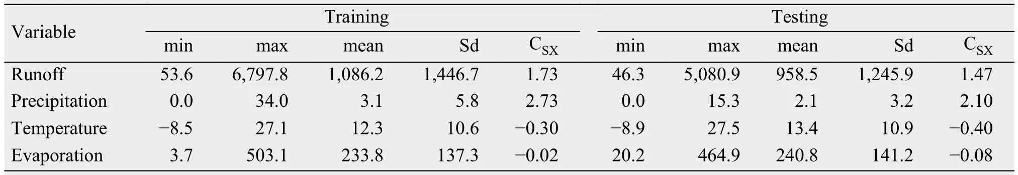
Table 1 Statistical analysis of MAR, MAP, MMT, and MAE time-series data

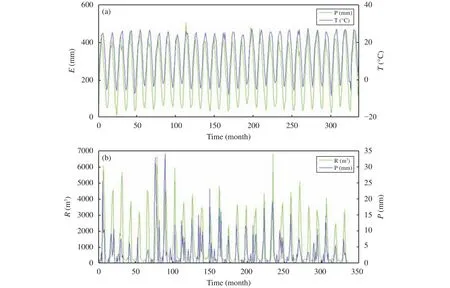
Figure 3 Time-series of (a) monthly average temperature and monthly accumulated evaporation and (b) monthly accumulated precipitation and monthly accumulated runoff

3.2 Model structure and output

The three-layer BP neural network (p, m, n) was used to train the CWNN and TANN models, where p,m, and n are the number of neurons in the input, hidden, and output layers. The RBFNN model increases the number of hidden-layer neurons gradually, which can increase the prediction performance of the neural network from relatively few conditions. The number of hidden-layer neurons in the RBFNN model can be determined when the results of the model are obtained. Therefore, the number of RBFNN hidden-layer neurons is not listed in Table 2 below. During the neural network training, the network parameters were set in advance, and the model error was obtained through network forward propagation. The error signal obtained in the previous step will propagate from the output layer to the input layer to adjust the parameters in the model. This process will continue until the network output matches the preset target. In this cycle, because the gradient algorithm is simpler than other algorithms, it is applied to the network-training process. The maximum number of training cycles, the performance goal (MSE), and the learning rate were set to 1,000, 0.01, and 0.01, respectively. The training process for the CWNN and TANN models used one neuron (m = 1) in the beginning, and then the number of neurons gradually increased. Finally, the optimal number of neurons was selected as the training structure of the model. As shown in Figure 3b,MAR, as the predicted variable, had strong periodicity. Therefore, the time of the predicted MAR also served as an input variable for the model. Through the computational simulation of the neural network, the training and prediction accuracy of the network could be generally improved when time was used as an input variable. The training results of the three neural network models are listed in Table 2.

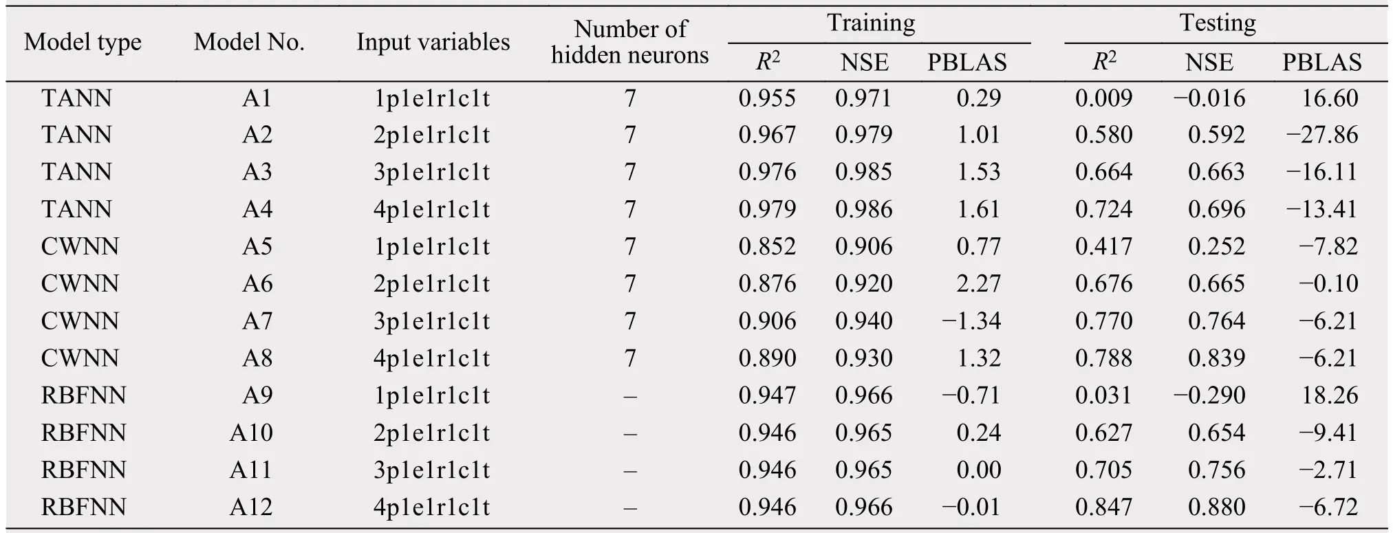
Table 2 Evaluation results regarding the model performance of TANN, CWNN, and RBFNN

Generally, the results indicated that the training and prediction accuracy of TANN and CWNN can be quickly improved when the hidden-layer neurons are gradually increased. If the number of neurons increases to 6 or 7, the accuracy of the model decreases rapidly. To intuitively compare the results of the different models' training, the number of neurons in the hidden layer was set to 7. The performance of TANN's training results was the best among the three models, but its prediction results were the worst.Meanwhile, the performance of CWNN's training results were the worst among the three models, but its prediction results were close to the training results of RBFNN. The results showed that TANN can be studied efficiently with input variables, but the simulation accuracy is low due to too many learning-sample details. Although the learning efficiency of CWNN is relatively low in the training stage, it can accurately reflect the internal rule of the sample data, which gives the model a higher prediction accuracy. Other important information provided by the results presented in Table 2 is that the training and prediction accuracy of each model can be significantly improved when the input variable increases the amount of MAP in different months. It is indicated that the MAP is strongly correlated with the MAR. Finally, it is shown that RBFNN performs better in both training efficiency and prediction. In short, RBFNN is more suitable as the prediction model for MAR.

3.3 Model-generalization improvement

Previous analyses have shown that the causes influencing neural network model training and prediction performance are multifaceted. To improve the training and prediction accuracy of the model, the model can be adjusted in many aspects. First, the appropriate model-error target (MSE) can be set up for different network models, which can effectively avoid the overlearning of the model and improve its prediction accuracy. Second, the number of appropriate hidden-layer neurons can be set to improve the ability of the model to learn the sample information, and effectively improve the accuracy of the model prediction.Finally, selecting variables that are strongly correlated with predictive variables and excluding variables that are independent of prediction variables are key to improving the model's training and prediction accuracy. The results of the variable selection are shown in Table 3 below, and all the experimental results are listed in Tables 4-6.

Through the adjustment and selection of the number of input variables in the neural network, the wavelet basis function of the hidden layer, the number of hidden-layer neurons, and the model-error target, the precision of neural network training and prediction was greatly improved. From the experimental results listed in Tables 4-6, all three neural network models have good training and prediction performances. The next step, then, was to select the three best-performing models (B4, C6, and D8) to train and predict the MAR one month in advance. To visualize the results of the three model predictions, we use regression plots(Figure 4). For a perfect prediction model, all the data should fall along a 45° line of the plot, which is the output of the model equal to the target observation.High correlation coefficients [R = 0.903 and 0.901 for ANN B4 (Figures 4a, 4b); R = 0.880 and 0.901 for CWNN C3 (Figures 4c, 4d); and R = 0.918 and 0.906 for RBFNN D8 (Figures 4d, 4f)] were found in the model-training and -prediction stages, indicating that the fitting data were reasonably good.

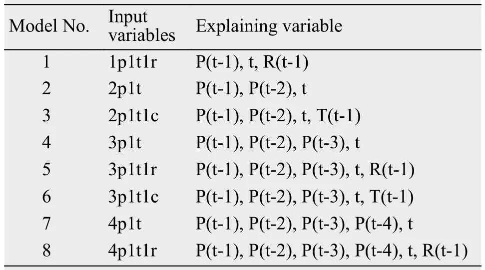
Table 3 Input structure of the ANN, WNN and RBFNN models for runoff modelling

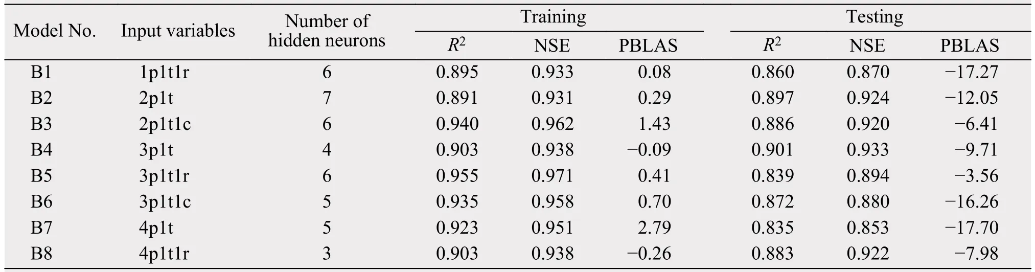
Table 4 Evaluation results of the TANN model's performances

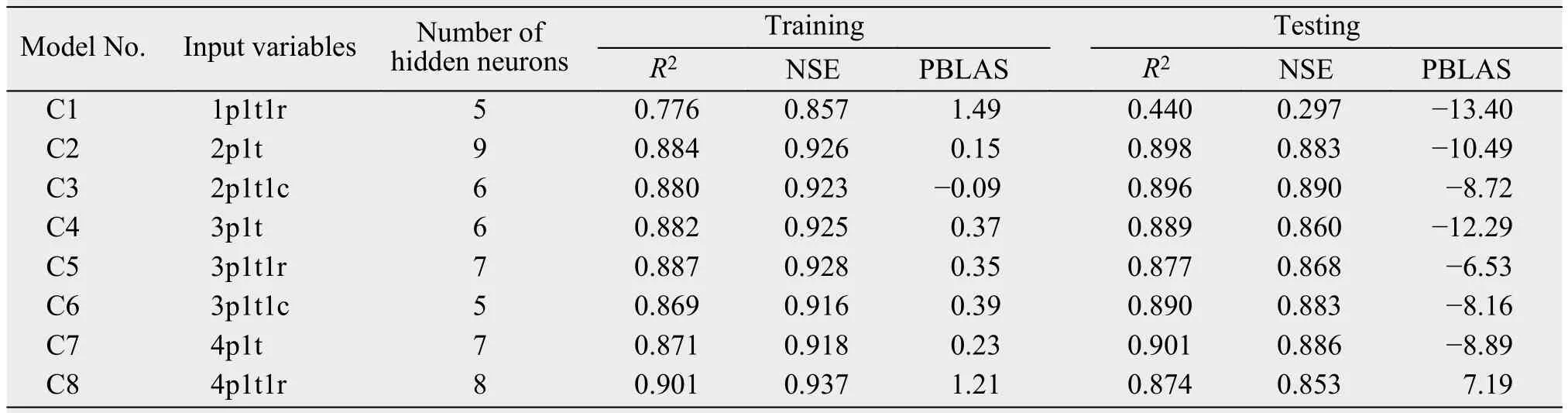
Table 5 Evaluation results of the CWNN model's performances

Comparing the performance indicators of the three models' (B4, C3, and D8) prediction stages, it was found that each model performs excellently in this stage. However, compared with CWNN C3, TANN B4 and RBFNN D8 performed better in capturing runoff peaks (Figure 5). The height of the runoff peaks simulated by TANN B4 is basically the same as that shown in Figure 5a. It shows that the TANN model duplicates the periodic variation of MAR mechanically, and the mapping relationship between the input variables and MAR is not accurately found during the model's training phase. The MARs in the neural network training phase (1981-2000) and the prediction phase (2001-2008) show a relatively large difference (the MAR decreased by 13.3% during the testing phase). Tables 4-6 show that the PBIAS in the testing phase was basically around -10 (the predicted value was more than 10% of the observed value).

The TANN model performed well both in the training and prediction stages, but it is not suitable as a predictive model for MAR. The reason is that the TANN model learns more sample details and cannot effectively reflect the underlying rules of the data,meaning the simulation stage cannot capture the peak of MAR effectively (Figure 5a). From the data in Table 4, the accuracy of the CWNN model in the prediction phase was the closest to the training accuracy among the three models. This shows that the CWNN model has a natural advantage in predicting data with random vibration or periodic changes. In previous studies, the performance of the CWNN model in simulating runoff was found to be the best among all models, whereas in this study the performance was not as good as that of the TANN and RBFNN models(Nourani et al., 2009a,b). The main reason is that the predictive variables are set to change in the small interval among previous problems; however, the CWNN model could capture the overall law of data changes effectively. Unfortunately, our study area, being an arid-oasis landscape, means that the runoff flowing through the oasis area experiences huge change from the dry season to the wet season. The predicted variable (MAR) fluctuated greatly in a short period of time (12 months), making the model unable to analyze effectively the information in the sample data, which is an important reason for the poor training results of the CWNN model.

Table 6 Evaluation results of the RBFNN model's performances

4 Conclusion

The Qira River Basin originates in the high-altitude valleys of the Kunlun Mountains. Therefore, the precipitation in the Kunlun Mountains is the main factor affecting the river's runoff. There are no longterm meteorological or hydrological stations in the Kunlun Mountains, which is a major obstacle for the collection of data affecting runoff. In this study, to train and forecast the MAR of the Qira River, we relied on two scientific stations in the middle and lower reaches of the Qira River to collect relevant data that influence runoff.

By comparing the prediction results of several neural networks, we can conclude that the three neural network models possess good training and prediction accuracy, and can accurately capture the appearance of the peak flow. Each neural network model has its own characteristics and advantages. For instance,the CWNN model has superior learning ability, with stochastic fluctuation and cyclical variation of data.Indeed, previous studies have shown that the CWNN model performs well in the simulation of rainfall runoff, as compared with other models. That said, studies have tended to be in areas with low altitude and dimensionality, where the main form of precipitation is water rather than snow; plus, the rainfall is relatively more balanced throughout the year. For arid-oasis regions like in our study, the runoff flowing through the oasis originates in a high-altitude area; and the MAR of the Qira River changes dramatically throughout the year. Our numerical experiments showed that, although the CWNN model has advantages in capturing the random fluctuation of data, the training accuracy is not high when faced with data characterized by large fluctuation over a relatively short period. The TANN model, meanwhile, is prone to overlearning during the process of network training, resulting in a poor accuracy of data prediction in later stages. This makes it necessary to spend a lot of time on the process of using the TANN model to find the appropriate model-error target and hidden-layer neuron number. All kinds of variables in the TANN and CWNN models require the computer to randomly set the initial value at the initial training stage. These models, as is typical of BP neural networks, are very sensitive to the selection of their initial parameters. Therefore,when the optimal goal, the number of hidden-layer neurons and appropriate model-error target have been confirmed, they also need to simulate the model several times to find the optimal model output. Therefore, a new BP neural network that can be trained to achieve convergence is also closely related to the capacity of the training sample, the choice of algorithm,the network structure of the predetermined nodes (input nodes and hidden-layer nodes, output nodes, and the transfer function of output nodes), the expected error, and the number of training steps. At present,many RBFNN training algorithms support online and offline training, which can dynamically determine the data center and extended constants of the network structure and hidden-layer unit. The learning speed is faster than that of the BP algorithm and shows better performance. Besides, the TANN model is more demanding than the RBFNN model in terms of the selection of input variables. It also takes a long time to select variables. Therefore, the RBFNN model has more advantages than the TANN model and CWNN model. In short, the RBFNN model is more suitable for the study of runoff prediction in arid areas.

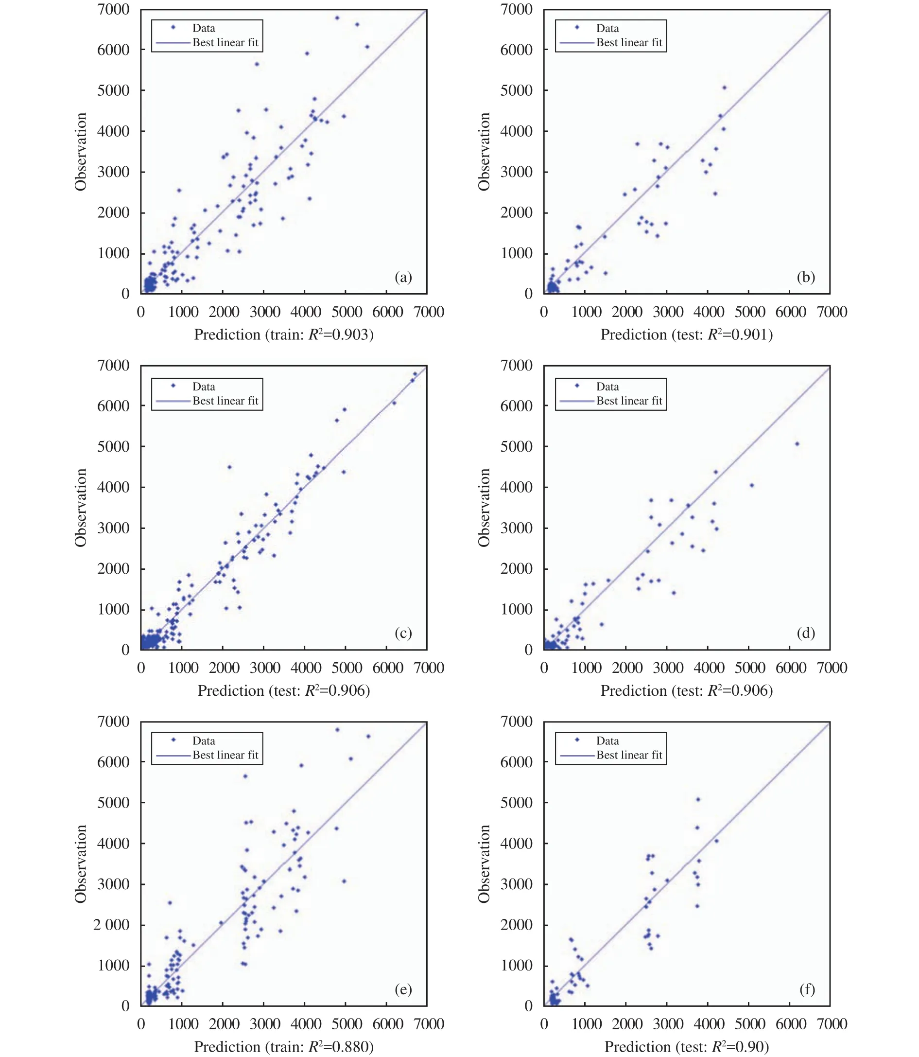
Figure 4 Regression plots displaying the training and testing results of the TANN model B4,CWNN model C3, and RBFNN model D8

Figure 5 Comparison of observed data and predictions for the (a) TANN model B4,(b) CWNN model C3, and (c) RBFNN model D8

From 2001 to 2008, the study area experienced significant climate change. The precipitation in the Kunlun Mountains area decreased significantly. The decreasing precipitation increases the uncertainty of the model in the prediction process, making it increasingly difficult for the neural network to capture the position of the runoff peak. This result was caused by there being no data available on precipitation in the Kunlun Mountains and the utilization of the relevant Qira River precipitation data instead. Using the RBFNN model to simulate the Qira River can accurately reflect the MAR of the next month. In summary, the results of this study provide a useful reference for risk assessment in the Qira River Basin, as well as in the decision-making process of water-resources management and planning. Similarly, there are oases of different sizes along the northern foot of the Kunlun Mountains. The ecological environment and geographical structure of these oases are very similar to those of the study area focused upon in this paper.These oases are overly dependent on reclaiming oases to maintain regional development. There is no scientific basis or data reference for the management of their water-utilization systems. As such, we can provide a better decision-making basis for oasis development by enhancing the study of runoff throughout the region.

Acknowledgments:

This work was financially supported by the regional collaborative innovation project for Xinjiang Uygur Autonomous Region (Shanghai cooperation organization science and technology partnership project) (2017E01029), the "Western Light" program of the Chinese Academy of Sciences (2017-XBQNXZ-B-016), the National Natural Science Foundation of China (41601595, U1603343,41471031), and the State Key Laboratory of Desert and Oasis Ecology, Xinjiang Institute of Ecology and Geography, Chinese Academy of Sciences (G2018-02-08).