A Computer-Aided Tuning Method for Microwave Filters by Combing T-S Fuzzy Neural Networks and Improved Space Mapping

Shengbiao Wu , Weihua Cao , , Can Liu and Min Wu

Abstract: A computer-aided tuning method that combines T-S fuzzy neural network (TS FNN) and offers improved space mapping (SM) is presented in this study. This method consists of three main aspects. First, the coupling matrix is effectively extracted under the influence of phase shift and cavity loss after the initial tuning. Second, the surrogate model is realized by using a T-S FNN based on subspace clustering. Third, the mapping relationship between the actual and the surrogate models is established by the improved space mapping algorithm, and the optimal position of the tuning screws are found by updating the input and output parameters of the surrogate model. Finally, the effectiveness of different methods is verified by an experiment with a nine order cross coupled filter. Experimental results show that, compared to a back propagation neural network method based on electromagnetic simulation and an SM method based on a least squares support vector machine, the proposed method has obvious advantages in terms of tuning accuracy and tuning time.

Keywords: Computer-aided tuning, T-S FNN, S-parameters, coupling matrix.

1 Introduction

With the development of electronic technology and wireless communication techniques,the demand for frequency selection of microwave filters is increasingly expected [Hunter,Billonet and Jarry (2002)]. The methods for improving the inhibition ability of the microwave filter and reducing the loss capacity of the passband have attracted attention of engineers. However, in actual application, because of the differences between the mechanical error and the material characteristics of the microwave filter, the output response based on the electromagnetic design have fallen short of theoretical expectations[Xu, Yong and Zhang (2013)]. This is an urgent problem for wireless and satellite communications, the requirements for which are particularly strict. Because the manufacturing tolerance of the filter does not leave sufficient space for design allowance,the tuning has become critical.

Over the past few years, the tuning methods for filters have been mainly based on artificial tuning which not only consumes considerable time and effort but also affects the consistency of products [Michalski (2010)]. To improve the efficiency of production, an intelligent tuning method based on least squares support vector machine (LS-SVM) was presented [Zhou, Duan and Huang (2011)]. This method develops a means of tuning directions by combining the tuning model and optimization strategy. However, this method ignores the effect of parameter extraction on system performance. To solve this problem, a computer-aided tuning system for microwave filters was developed [Yu(2011)]. To its credit, the tuning device can be flexibly changed and screws can be finetuned. However, this method is limited when it is used for microwave filters with different topologies. Subsequently, a neural network with SM optimization of microwave filters was proposed in Wang et al. [Wang, Yu, Kabir et al. (2012)]. This method not only applies the back propagation (BP) neural network to filter tuning, but also realizes computer-aided tuning through surrogate parameter optimization. However, it cannot be applied to actual filters. In Zhang et al. [Zhang, Su, Liang et al. (2013)], the Cauchy method was used for parameter extraction, but the initial value of both the optimization variables and convergence region was not considered, which means the system is hard to converge.

In 2014, the improved time domain tuning method was proposed in Song et al. [Song,Zhang and Cao (2014)], where the resonant frequency and coupling coefficients could directly reflect the characteristic changes of output waveforms of microwave filters. This method can direct the tuning of the filter intuitively and quickly, however, it can hardly be applied to cross coupled and higher order filters. Therefore, a tuning based on the phase meant for coupled resonator filters was proposed [Ness (2015)]. Here, the tuning direction of the filters was directed by iterative optimization to minimize the error between the output phase of each tuning and the ideal phase responses. This method can avoid the convergence problem of optimizing the parameters, however, the tuning process is very complex.

Multi-objective optimization methods based on Daubechies D4 wavelet transform,Hausdorff distance, and Frchet distance were proposed by Michalski et al. [Michalski,Gulgowski and Kacmajor (2012); Kacmajor and Michalski (2012); Szwaba, Forest and Kacmajor (2016)], but these methods are difficult to apply to multi-order cross coupled microwave filters. To improve the efficiency of tuning, a multi-dimensional optimization method based on a surrogate model was proposed by Xia et al. [Xia, Ren and Choi(2017)]. This method realizes optimizes parameters successfully by employing the electromagnetic simulation model. In [Mohammed, Bouhafs and Rachid (2018)], an antenna optimization design and simulation experiments were conducted using the library function HFSS-MATLAB-API of MATLAB, and a 3D model was generated by HFSS software. To a certain extent, this approach is convenient for optimization design and theoretical simulation of the size of the microwave filter. However, uncertainties remain with the mechanism of electromagnetic simulation software.

A computer-aided tuning method that combines a T-S fuzzy neural network (T-S FNN)and improved space mapping (ISM) is developed in this study. The significance of this method is threefold: i) Coupling matrix (M) extraction in a non-ideal state is realized after initial tuning; ii) Surrogate modeling based on field tuning data can be applied to microwave filters with different topologies, and data clustering and the self-learning of model parameters enhance the prediction accuracy of M; and iii) Configurations of the convergence radius and update mode make the tuning process simple and fast. The remainder of this paper is organized as follows. Section II describes in detail the design of the tuning scheme. Section III presents the method of primary tuning through an optimization design. Section IV introduces the phase shift and extraction processes of coupling matrix. Section V describes the verification of the surrogate model and computeraided tuning through experiments. Finally, Section VI presents the conclusion to this study.

2 Description of filter tuning

2.1 Structure of the model

The structure of the actual and the surrogate models are shown in Fig. 1. The left half of Fig. 1 shows the extraction process of the coupling matrix, which consists of three main parts: First, the scattering parameters (S-parameters) without phase shifts are collected and converted into admittance parameters (Y-parameters). Second, the poles and residues of Y-parameters are extracted by the vector fitting method. Third, the coupling matrix is extracted by comparing the expression of Y-parameters. The right half of Fig. 1 presents the realization of Mto S-parameters. By establishing the mapping relationship between the surrogate and actual models, the screw height can be obtained through iterative optimization.

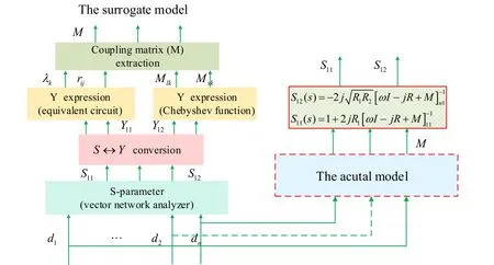
Figure 1: Surrogate and the actual models

2.2 Tuning process of filter

The core task of computer-aided tuning is to establish a surrogate model based on field data and realize parameter optimization. A thorny problem in this task is to extract the M from the S-parameters under non-ideal conditions. However, the coupling matrix cannot be extracted when the S-parameters curve is distorted. Therefore, the error of the output response should be adjusted to the allowable range by the initial tuning of the filter.Fig. 2 shows the specific tuning process, which mainly includes four pieces of information: First, the zero-poles location optimization of the initial tuning is presented;Second, the coupling matrix is extracted by vector fitting in the presence of phase shift and cavity loss; Third, the T-S FNN is used to establish the surrogate model based on field data; Finally, the iterative optimization of ISM is used to find the optimal position of the screws.

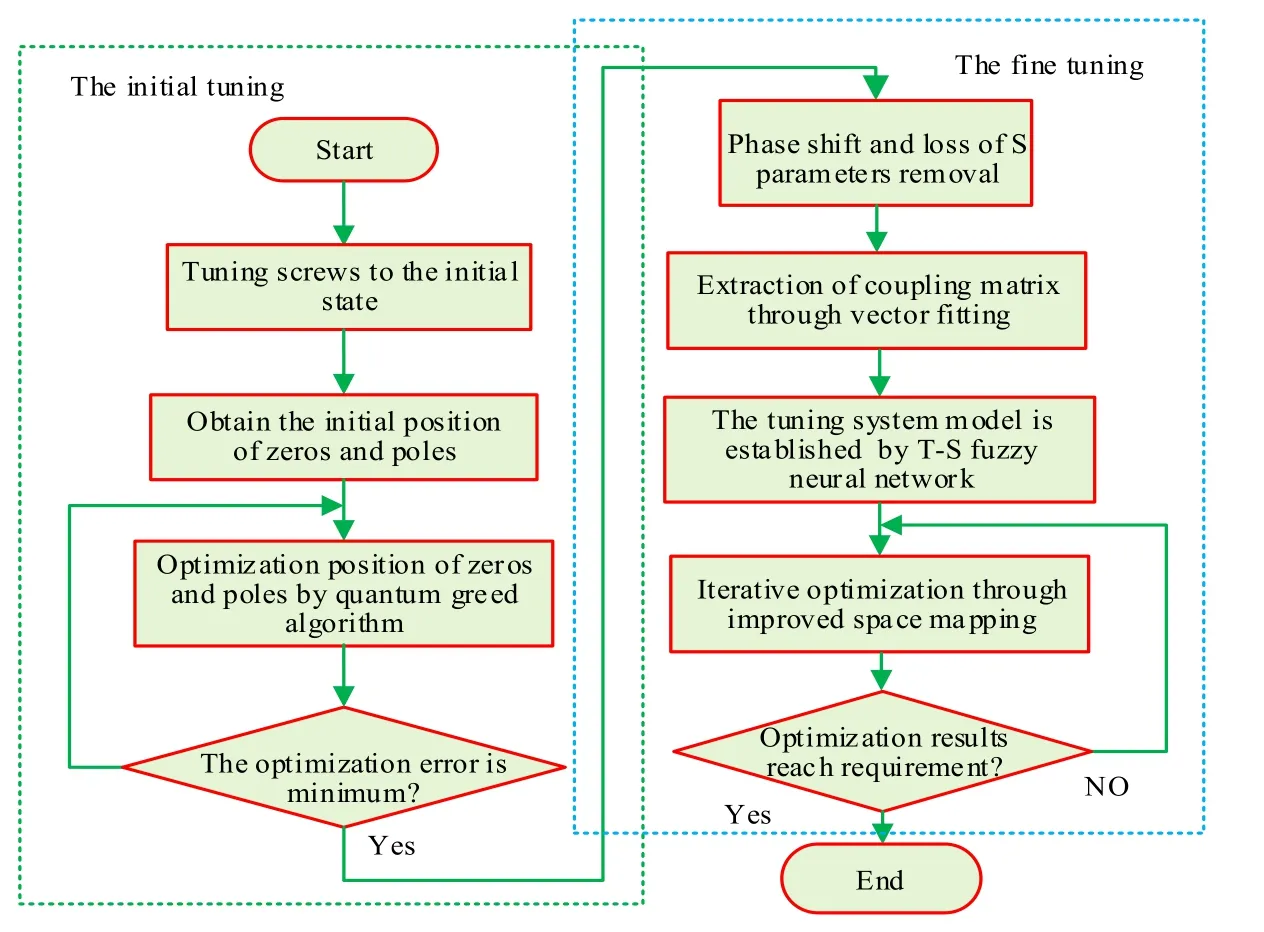
Figure 2: Computer-aided tuning flow of the microwave filter

3 Initial tuning of the filter

The goal of initial tuning is to tune the S-parameters to a reasonable range to enable smooth extraction of M. To achieve this goal, optimizing zero-poles location is essential.The expressions of the transmission (S12) and reflection functions (S11) of the filter are given as follows:

where RL is the return loss; Nzand Nsare the number of zeros and poles, respectively;and k3are weights, and the position of the zeros and poles are patched by a greedy algorithm. Here,z11k, z21kand pkare set as optimization variables. The optimization target is realized when the value ofapproaches zero [Sujatha,Ramakrishnan and Duraipandian (2014)]. To avoid the system falling into local extremum and precocity, this study integrates individual, social and excellent individual knowledge in quantum updating [Yang, Peng and Cao (2014)]. The expression is as follows:

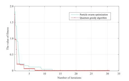
Figure 3: Comparison of the fitness of different algorithms

Fig. 3 shows the number of iterations and error precision curve of the network are shown in Fig. 3. As shown, the precision of the quantum greedy algorithm can reach 0.232 after eight times of training. When the traditional PSO algorithm is used, 13 times of training can reach 0.896. The quantum greedy algorithm is obviously better than the traditional PSO algorithm.

Figure 4: Iterative error of the S11

Fig. 4 and Tab. 1 present the iteration error of S11, whererepresents the characteristic error. As the number of iterations increases, the error of S11between the extracted and ideal indices becomes smaller, but approach zero is difficult. Therefore, the filter requires further tuning to meet performance requirements.

Table 1: Extracted error characteristics of S11

4 Extraction of coupling matrix

The physical structure of the filter is generally designed with resonators and coupling cavities, where each cavity is equivalent to a parallel resonator circuit. Fig. 5 shows the one-to-one correspondence between the coupling matrix and tuning screws. Here, we can see that when the tuning magnitude and direction of the screws are changed, both the value of the coupling matrix and the S-parameter produced by the coupling matrix are changed. Therefore, the extraction of the coupling matrix is an essential part of filter tuning. The specific extraction process is described as follows.

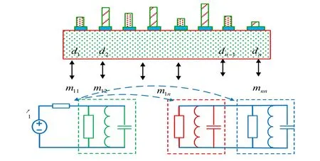
Figure 5: Corresponding relationship between M and tuning screws

4.1 Removal of phase shift

Unlike the ideal filter designed using HFSS software, the S-parameters of the actual filter contains a phase deviation be produced by the transmission line, cavity loss and high order mode. If this phase deviation cannot removed effectively, it will affect the extraction of the poles and residues, which in turn affects the synthesis of the coupling matrix and the establishment of the later surrogate model. Therefore, the phase deviation must be removed, it is the expression for which is as follows [Macchiarella (2010)]:

It is assumed that the phase loading and length of the transmission line at the two ports are equal, or in other words:Thus, the phase deviationofmust be removed. Based on Zhang et al. [Zhang, Su and Wu (2013)], the phase expression of S11is as follows:

where cnand enare the polynomial coefficients of the numerator and denominator,respectively. Whenis satisfied, the formula can be translated as follows:

where a and b are proportional constants. The phase and group delay of S11after the phase is removed is as follows:

Figure 6: Amplitude of Y21 before and after phase removal

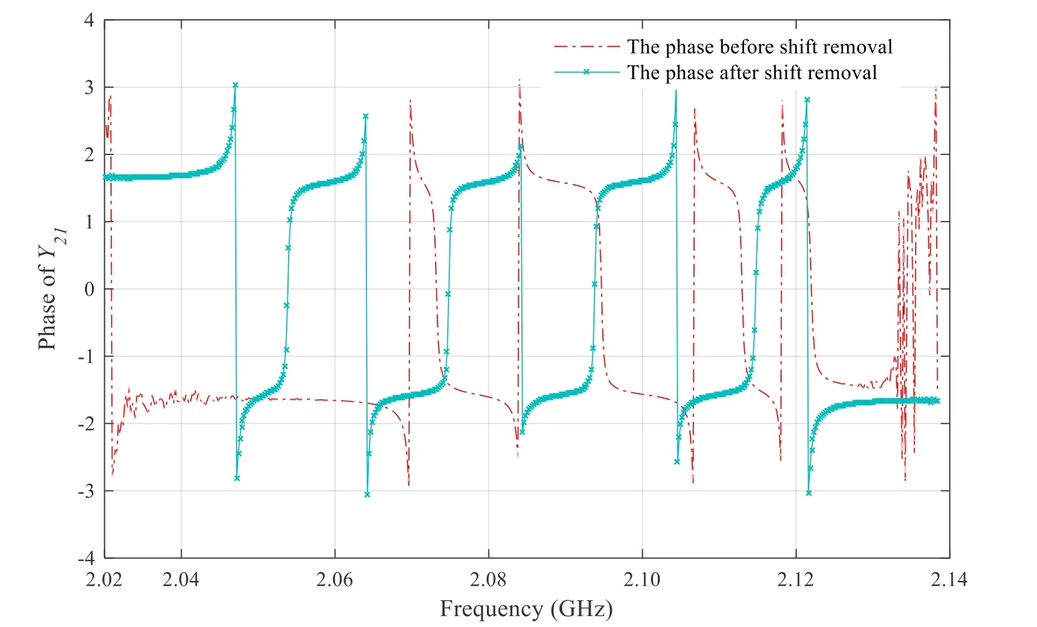
Figure 7: Phase of Y21 before and after phase removal

Based on the aforementioned expression, the scaling factor can be calculated by curve fitting. After fitting is completed, the phase loading of ports 1 and 2 areandrespectively. In addition, the transmission line length is 3.1462e-9 m and 4.0112e-9 m, respectively. From the amplitude of Y21in Fig. 6 and the phase of Y21in Fig. 7, we can clearly see that the curve after phase removal can be approximately centrally symmetric, and expression of transmission and reflection characteristics after the phase deviation is removed is as follows:

where1φ and2φ are the phase shift caused by the transmission line;and Sijare the S-parameters before and after phase shift removal. The Y-parameters can be obtained by the new S-parameters. Once the poles and residues of the Y-parameters are calculated by vector fitting, the coupling matrix can be easily synthesized.

4.2 Calculation of poles and residues

After the phase deviation of S-parameters is removed, the poles and residues of Yparameters can be calculated by vector fitting. In this study, to avoid the dependence of the fitting process on initial poles and residues, the initial poles are obtained by least squares before the vector fitting. The formula for converting the S to Y-parameters is given as follows [Meng and Wu (2016)]:

The advantage of using vector fitting is that it not only avoids the problem of high power in the polynomial coefficients extraction, it merely iterates the previous poles and remainders to the next step. Thus, the process is relatively simple and rapid. The expressions of the Y-parameters shown by the poles and residues are as follows [Goay,Goh, Ahmad et al. (2018)]:

In the formula, n and k are the number of the order and sampling points, respectively.To obtain the poles and residues, the formula must be further converted as follows:

Formula (12) is treated as a form of, and the unknown elementcontaining the poles and residues must be solved. When the value of σ(s) approximates 1, the poles and residues can be calculated. Tab. 2 shows the results.

Table 2: Extracted poles and residues of the Y-parameters

4.3 Coupling matrix synthesis

When the adjustable variables of the microwave filter are large, a single optimization method is considerably dependent on the initial value. Therefore, the analytical method based on vector fitting is crucial for the extraction of the initial M. Considering that the number of transmission zero points is far less than the order of the microwave filter, the formula. From the synthesis of the Chebyshev function and the equivalent circuit of the coaxial cavity filter, we can derive the following formula [Wang, Li and Peng (2015)]:

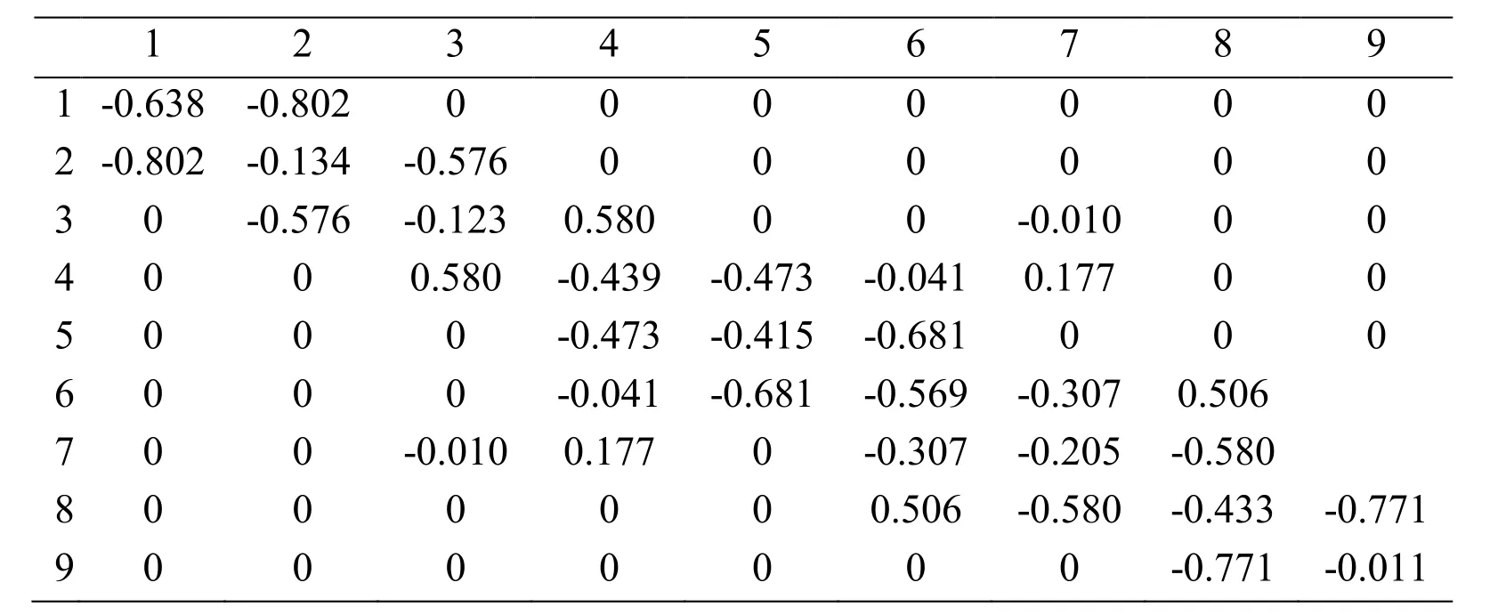
Table 3: Extracted M of the nine order cross-coupled filter

5 Surrogate model and the computer-aided tuning

The FNN based on the T-S model combines the advantages of the fuzzy reasoning ability and the self-learning of a neural network [Zhang, Jiang, Yin et al. (2018)]. In this study,the T-S FNN is used to build a coupling matrix prediction model. The prediction value is then fed into the ISM. Finally, the optimal tuning position of the screws is found by iterative update of the input and output parameters of the surrogate and actual models.

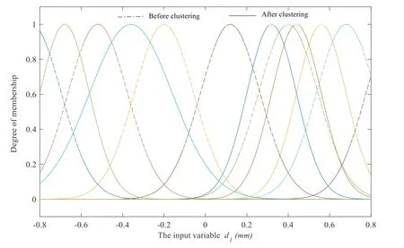
Figure 8: Membership function of d1 before and after clustering

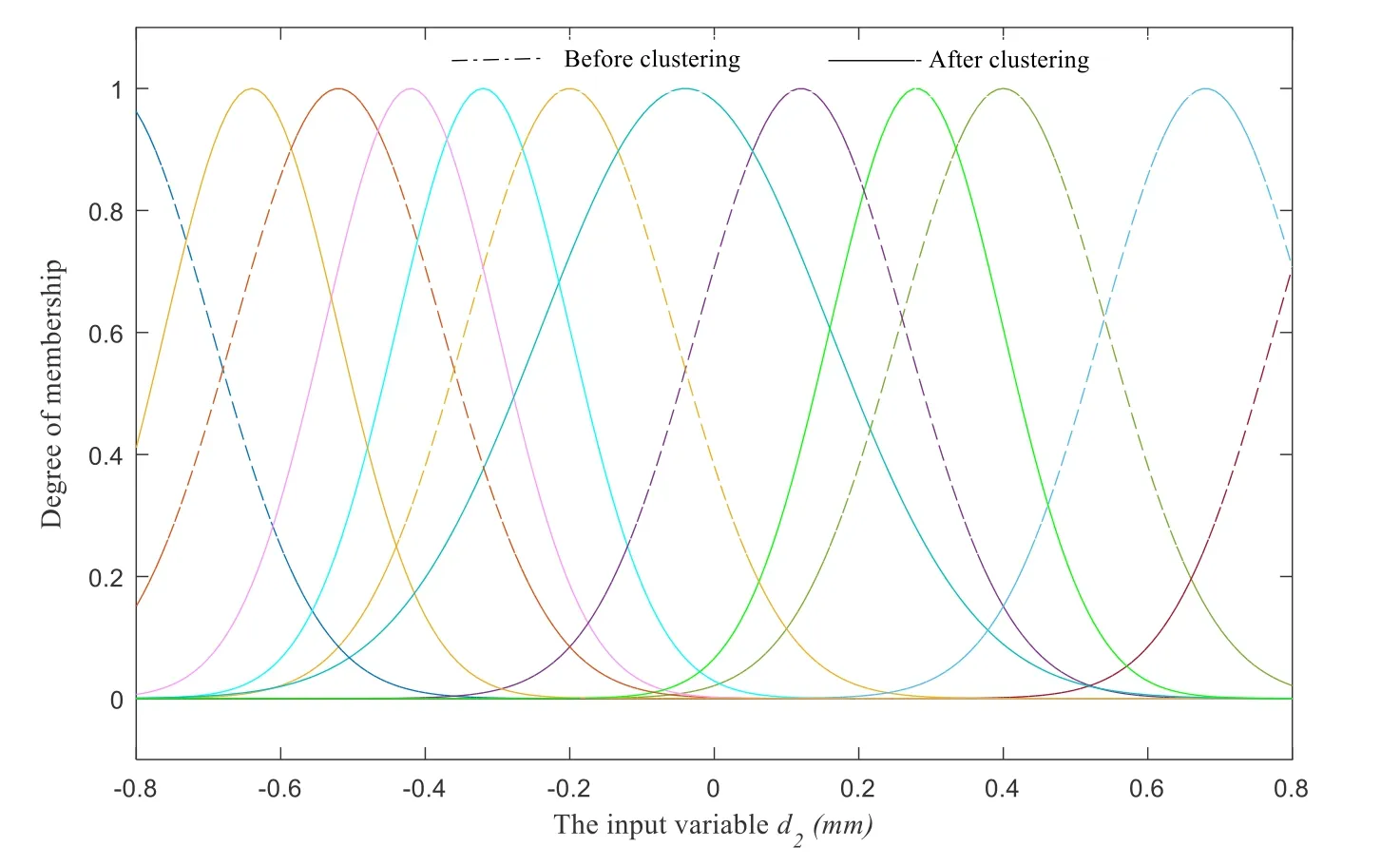
Figure 9: Membership function of d2 before and after clustering

Compared to the tuning method based on the 3D model built using HFSS software, the method has faster convergence speed and higher prediction accuracy.

5.1 Fuzzy clustering

To improve the effectiveness of empirical data, the fuzzy C-means clustering (FCM) is used to partition the input space of FNN based on the T-S model, and the cluster centers are calculated through subtractive clustering based on the density around each data point.To reduce the influence of different dimensions on the model, the input and output data must be normalized to [ ]0 1 [Castro, Fronza and Alves (2017)]. The fuzzy clustering is realized by the following procedure.

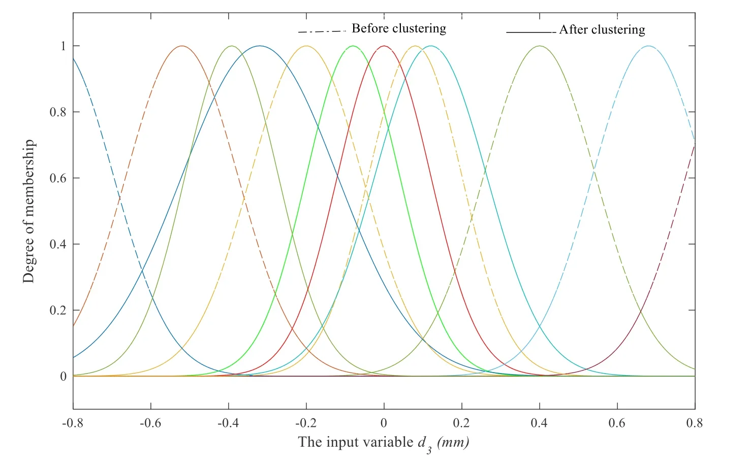
Figure 10: Membership function of d3 before and after clustering

Step 1: According to the subtractive clustering formula, the density index of data points at xiiswhereis the neighborhood radius of the data point, and the density index of every data point can be updated by using the following formula. Where xiis the density index at the center data point, and to avoid a near clustering center, we set

Step 2: Based on the FCM criterion, the minimum cost function is transformed into the following equation.

wherekjμ is the membership of the sample data j belonging to the class k and Vkis the center data of the class k. The optimal conditions for the aforementioned equation are as follows.

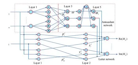
Figure 11: Structure of T-S FNN

Step 3: The number of the clustering and initial clustering center are obtained by subtraction clustering by the following equation:

The subdivision of input data before and after clustering is shown in Figs. 8-10. The real and dashed lines in the graph represent the membership functions of input data before and after clustering, respectively. Clearly, the data after processing can truly reflect the tuning rule of the system. It provides considerable help for modeling the tuning system.

5.2 Structure of T-S FNN

The T-S FNN is mainly composed of forward and post networks. The primary aim of the front network is to match the fuzzy rule, and the aim of the post network is to produce the fuzzy rule [Le and Hai (2016)]. Fig. 11 shows the structure and relevant parameters of the network.

The input layer of the forward network is, and the Gauss type functionis adopted as the membership function layer. The number of fuzzy rules is equal to the number of central values of the network, where. The outputs of the last two layers isandrespectively. The purpose of taking x1=1 in the first layer of the post-network is to calculate the constant term. The post parameters of each rule are calculated on the second layer, and the output values of the last two layers areandrespectively.

5.3 Parameter identification of T-S FNN

To strengthen the effectiveness of the surrogate model, adaptive learning is conducted for parameter identification of the forward and post networks [Djelloul, Sari and Latreche(2018)]. The updating formula of the weight value is as follows.

where i, qand m are the number of input variables, output variables and training samples, respectively. Here, α=0.85 is a weighting coefficient selected in accordance with training and test errors. The following formula shows the online self-learning method of the central value:

The width value of membership functions can be identified online by the following iteration.

where miis the number of membership functions for the ith input,andare the width of membership functions corresponding to t+1 moments and t moments,respectively.is the width change of the membership function. Similarly, the objective function of the network training is designed as follows.

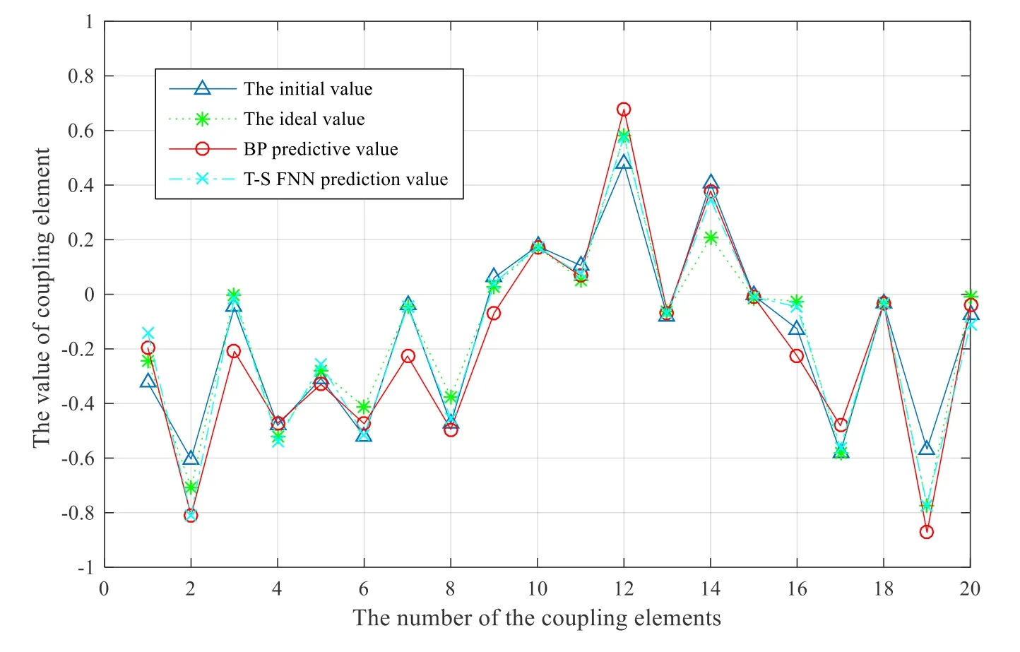
Figure 12: Prediction value of the coupling matrix by T-S FNN

where Mqandare the predicted and true values of the M, respectively, β represents the weighting coefficient selected based on training and testing errors,iω denotes the parameter values that must be adjusted in the front and rear parts of the T-S fuzzy neural network. As Fig. 12 shows, compared to the conventional BP neural network method, the extraction precision of M is more accurate, and the purpose of prediction can be achieved when the initial tuning of the filter is completed.

5.4 Computer-aided tuning

Traditional tuning is normally achieved by optimizing of its own parameters. Traditional tuning has slow tuning speed, is sensitive to the initial value, and is particularly powerless to high order filters. For these reasons, the space mapping algorithm is used to establish relations between the surrogate and actual tuned models. Obtaining the best tuning position of the screws by optimizing the parameters of the surrogate model is easy.Because of the number of variables in the system, the radius of the confidence domain and the initial Jacobian matrix are improved on the basis of the space mapping algorithm.For convenience of operation, the input variables are represented asandin the surrogate and actual models, respectively. The corresponding S-parameters are expressed byandrespectively, where, n is the order of the filter and k is the number of iterations. i=1,2, j=1,2. Using the improved algorithm, we could find the appropriate position of screws that meets the performance index. The solution of the location of the screws is transformed into the following optimization problem [Wang and Zhang (2012)]:

Step 1: Obtain the optimal coupling matrixunder the best Sparameters of the nine order coaxial cavity filter. Set the value of the initial Jacobian matrix.

Step 3: Calculate the error betweenandifexists , the solution

for the system is derived from the height of the screws obtained at this time. Otherwise,execute the next step.

Step 4: If the error is not within the allowable range, update the tuning height of the screws using the formulawhere h(k)is obtained by combining ofand

Step 5: Set the radius γ of the confidence region. Let. If the value of the equationis less than or equal to ζ, terminate the tuning program.

Step 6: Update the iteration number k=k+1. Then perform the following iteration in the same manner until the iteration precision approximates the permitted value.

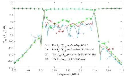
Figure 13: Comparison of S-parameters before and after tuning

Table 4: Extracted performance parameters of different methods

A comparison of S-parameters when using different the methods are presented in Fig. 13 and Tab. 4, where ILminrepresents minimum insertion loss; LR and RR represent left and right restraints outside the band, respectively; andand RLaverepresent the maximum, minimum and average return loss, respectively. We observe that the error of S-parameters made when combining the BP neural network and electromagnetic simulation (ES) is relatively large. The methods based on LS-SVM and SM make achieving the desired index requirements difficult as well. However, following several iterations by T-S FNN and ISM, the transmission attenuation of the passband in 2.06-2.14 GHz is less than l dB, the fluctuation is less than 0.5 dB, the reflection coefficient of the port is less than -40 dB, and the output response of the proposed method is in good agreement with the ideal curve.

6 Conclusion

Considering the difficulty and complexity of the tuning process, a computer aided tuning method based on T-S FNN and ISM was developed in this study. We showed that this method is effective at avoiding the inaccuracy of parameter extraction when the filter detuning is large, and it can overcome the effects of phase shift and cavity loss on the accuracy of Mextraction. In addition, the reliability of modeling was greatly improved by data clustering analysis and the self-learning of model parameters. In addition, the convergence speed of the optimization algorithm was obviously improved by setting the radius of the confidence region and initial value. The experiment of the nine order coaxial cavity filter showed that this method has good practical significance for the auxiliary tuning of filters.

Acknowledgement:This work was supported by the Hubei Provincial Natural Science Foundation of China under Grant 2015CFA010 and the 111 project under Grant B17040.