Testing and numerical simulation of a medium strength rock material under unconfined compression loading

Aria Mardalizad,Riccardo Scazzosi,Andrea Manes,Marco Giglio

Politecnico di Milano,Department of Mechanical Engineering,Milan,Italy

1.Introduction

This article presents experimental and numerical investigations in the rock mechanics domain with a focus on the oil and gas requirements.Comprehensive knowledge about the mechanical behaviours of rock materials in sub-aqueously deep well drilling applications is mandatory(Pepper,1954;Lacyand Lacy,1992;Brady and Brown,2013).The mechanical behaviour of rock at material scale is generally controlled by the geometric arrangements of the mineral particles and voids in combination with the microcracks.However,the micro flaws often significantly influence the rock mechanical behaviours(Åkesson et al.,2004;Szwedzicki,2007;Basu et al.,2009).The failure modes of brittle crystalline rock materials under compression loading are rather complex and difficult to be predicted (Santarelli and Brown,1989).This complexity originates from different sequential processes,which are discussed in this paper for the case of uniaxial compression loading(Martin,1993;Malvar and Crawford,1998;Li et al.,2003;Jaeger et al.,2007).Therefore,investigation on the failure mode of the rock material,a medium strength rock material(i.e.unconfined compressive strength(UCS)in the range of 40-80 MPa(Attewell and Farmer,1976))can advance our understanding and facilitate the future design in this domain.

The UCS is one of the most significant parameters to characterise the rock materials and it plays an important role in predicting the boreability of the material(Kahraman,2001;Ceryan et al.,2013;Nazir et al.,2013).Boreability is used widely in analysis,design and classification of rock materials and is expressed by the maximum principal stress that the material can sustain under uniaxial compression.Due to this,a precise approach for UCS measurement is necessary in most fields of rock mechanics.Basically,a cylindrical specimen loaded by two compressive platens in parallel to its main axis is considered conventionally as the configuration of unconfined compression test.This conventional test suggested by the standard ASTM D7012-04(2004)has its drawback,mainly due to the radial shear stressed generated at the contact interface when applying a compressive load.The undesired radial stresses appear due to different elastic properties of the steel of the testing machine platen and the rock specimen.Mogi(1966,2007)suggested another arrangement to design the specimen in order to address this problem.The experimental and numerical analyses in this context show that the Mogi’s suggested method can measure the UCS more precisely.The experimental results reveal that the variability of the results obtained by Mogi’s configuration is much lower than that of conventional configuration.Later,numerical simulations also confirm it when stress concentration is considered at the rock-steel(of compressive platen)interface using conventional configuration(Mogi,2007).

An alternative to expensive field testing is available due to the rapid development of numerical analysis technologyin conjunction with advanced computer facility.Several numerical methods have been recently employed(Kochavi et al.,2009;Anghileri et al.,2011;Jaime,2011;Wu and Crawford,2015;Zhao et al.,2016)for simulating the mechanical behaviours of quasi-brittle materials,e.g.concrete and sandstones.The finite element method(FEM)is the most commonly used numerical technique in the research fields as well as in industrial applications.The implementation of the FEM for solving the solid mechanics problems,which are analysed in the continuum domain,is still one of the most accurate numerical simulation techniques.The presence of highly distorted solid elements in the numerical modelling of fractured rock is often encountered,which is one of the main drawbacks of Lagrangian FEM.The smooth particles hydrodynamics(SPH)is a mesh-less Lagrangian method which can discretise a system as a number of particles(or “mesh-points”)carrying the field variables.The capability of the SPH method to cope with high distortion has been proved as the nodal connectivity is not fixed in this method(Anghileri et al.,2011;Olleak and El-Hofy,2015;Bresciani et al.,2016).However,the performance of the FEM in terms of accuracy and time consumption is generally higher than that when the SPH particles are used.Therefore,inspired by the study of Bresciani et al.(2016),an approach was implemented to take advantage of both the FEM and the SPH methods in exploiting the finite element software.

Exploitation of efficient and realistic constitutive models has become one of the essential tools in structural analyses.A material model,called Karagozian and Case Concrete(KCC)model,was used in this study.The KCC model was developed by Malvar et al.(1994,1996,1997,2000).Finally,the results of the numerical models were compared with the experimental data.

2.Experimental programme

The unconfined compression test is conventionally performed by applying axial load to a cylindrical specimen with a specific length to diameter ratio.Various arrangements have been developed to perform the unconfined compression tests as indicated in Fig. 1.The short cylindrical specimen represented as type 1 is in direct contact with the compressive platens,which is a configuration suggested by the ASTM standard.The different mechanical behaviours of the rock specimen and the steel of compressive platens result in radial shear stresses at their interfaces,which is a focus in this context.The two configurations represented as types 2 and 3 were developed to overcome the shortcomings of the type 1.

In the configuration type 2,various types of lubricants were basically applied at the interfaces to eliminate the friction forces.Due to the frictionless boundaries,it may seem that this configuration is a preferred one.The sample end conditions are principally plan,and the stress state will not vary throughout the specimen and the deformation can be considered homogeneous.However,during the testing,a number of vertical cracks propagate starting from the outer surfaces of the rock,which is induced by the intrusion of soft lubricator into the specimen(Mogi,2007).Therefore,the idea of using lubrication to produce frictionless boundaries is not practical.

The dog-bone specimen,represented as type 3,was suggested by Brace et al.(1966)to avoid extending the effect of a mismatch at the ends of the specimen into the region of the specimen where fracture occurs.The Brace specimen is however unsuitable for performing the unconfined compression test mainly due to two drawbacks:difficult fabrication procedure and presence of bending stresses.Therefore,Mogi(2007)proposed another configuration,represented as type 4,toovercome the shortcomings existing in the other configurations.The merits and drawbacks of the Mogi’s configuration will be discussed in Section 2.2.

The merits and drawbacks of the configurations types 1-4 under uniaxial compression conditions are summarised in Table 1.The present paper concentrates on two experimental testing programmes,i.e.types 1 and 4,as the methods of testing rock samples.

Fig. 1.Various configurations of rock specimens under uniaxial compression(Mogi,2007).

Table 1Merits and drawbacks of different arrangement types under unconfined compression(Mogi,2007).

The Mogi’s arrangement(type 4)was suggested to counteract the stress intensification at the interface between the steel plates and the specimen.Therefore,the Mogi’s configuration is expected to have two advantages with respect to the standard configuration:the precise determination of material strength,and the reduction of the variability of the material strength.

Rock failure modes are complex and difficult to be predicted.Several studies have been carried out in this regard;however,understanding rock breakage is still under investigation(Basu et al.,2013).Bieniawski(1984)suggested that physical models of the rock may provide useful information particularly when the failure modes are examined at laboratory scale,since there is no straightforward numerical(or mathematical)analysis model that can ascertain the nature of fracture development in rock materials.Based on the investigation of the failed rock specimens of sandstones and dolomite under triaxial compression tests,Santarelli and Brown(1989)concluded that failure can manifest itself in different ways depending on the microstructure of the rocks.A survey conducted on schist(anisotropic metamorphic rock),granite(brittle crystalline igneous rock)and sandstones(porous sedimentary rocks)by Basu et al.(2013)shows that rock failure mode in a uniaxial compression test may be one of the four types as shown in Fig. 2.

The uniaxial loading condition can impose tensile stresses on the specimens so that the cracks initiate and propagate from the tip of the microcracks and other defects when the tensile stresses exceed local tensile strength at that tip.These propagating cracks are called wing cracks.The predominant failure mode of the ASTM arrangement is expected to be axial splitting since wing cracks cannot be tolerated and eventually be aligned parallel to the maximum principal stress(Basu et al.,2013).However,the failure mode of the Mogi’s arrangement is supposed to be another type.When the wing crack propagation is inhibited,the coalescence of adjacent wing cracks,or of wing cracks in close proximity generated from the tips of suitably oriented microcracks,takes place in order to release the strain energy in the form of shear fracture.Therefore,it is assumed that the presence of the epoxycap stops the propagation of the wing cracks and thus,the specimen fails in the shear mode(Mogi,2007).

2.1.ASTM standard specifications

The first series of the unconfined compression tests was performed according to the protocols of the standard ASTM D7012-04(2004).According to the standard,the specimens must have a cylindrical shape with a length to diameter ratio,L0/D,between 2 and 2.5.The specimen diameter must also be greater than ten times the maximum grain size.According to Eni(2007),the sandstone is a medium-grained clastic sedimentary rock,with a sand size between 0.06 mm and 2 mm.The geometry data of the specimens are reported in Table 2.

The testing apparatus used for the standard configuration is shown in Fig. 3.The cylindrical specimen is compressed between two steel plates.The upper compressive platen(which is spherically seated)is displacement-controlled and the lower platen is fixed.The seating sphere must be properly lubricated and centred on the specimen faces.The seating sphere diameter should be greater than or equal to the specimen’s diameter but less than its double.The platens should have a diameter at least the same as the specimen’s diameter and a minimum of thickness to diameter ratio of 0.5.The upper platen should be displaced vertically at a constant rate of 0.1 mm/min.In this way,the time at specimen failure may occur between 2 min and 15 min as prescribed by the standard.An axial extensometer is placed at the mid-height of the specimen to measure the axial strain.Due to the presence of friction forces,the stress state can vary throughout the specimen and the deformation is thus not completely homogenous.Therefore,the gauge length of the axial extensometer used for the ASTM configuration is equal to 8 mm(less than 50%of the length of the shortest specimen)in order to guarantee that the axial deformation at this span remainshomogeneous.The applied loading amounts as well as the crosshead displacement were measured automatically by the testing apparatus.

Table 2Dimension of the specimens-the ASTM standard.

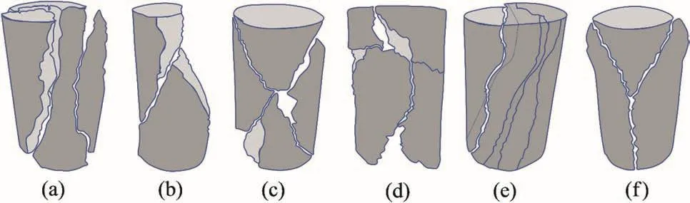
Fig. 2.Schematic representation of different failure modes under unconfined compression:(a)axial splitting,(b)shearing along single plane,(c)double shearing,(d)multiple fracturing,(e)failure along foliation,and(f)Y-shaped failure(Basu et al.,2013).

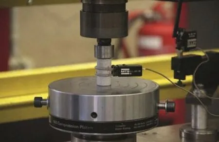
Fig. 3.unconfined compression test apparatus-the ASTM configuration.

2.2.Mogi’s enhanced layout

Due to the difference in the elastic properties of the platen steel of the testing machine and the rock specimen,radial shear stresses are generated at the contact interface after compressive load is applied.These stresses canproduce an undesired clamping effect at the end of specimen,which will raise two issues.The first one is that due to sudden shear stress transferring unexpectedly,stress concentration occurs at the specimen outer edge near the interface.The second is that if a crack propagates into the outer edge near the interface,the corresponding fracture growth is potentially prevented.These two issues may affect the true strength of a rock.As the stress concentration tends to decrease the strength,prevention of fracture growth tends to increase rock strength.However,the factors will almost never eliminate each other’s effect(Mogi,2007).

The drawback raised by the undesirable shear stresses can be significantly reduced by an enhanced arrangement designed by Mogi(2007)(see type 4 in Fig. 1).It consists of a cylinder connected to two aluminium end pieces by epoxy.The thickness of the epoxy is gradually decreased towards the middle of the specimens to form a smooth fillet in order to eliminate the stress concentration on the rock-steel contact interface.Nevertheless,it is not necessary to obtain the exact surface of the fillet since the epoxy has an elastic property lower than that of most rocks.

The main disadvantage of Mogi’s configuration is that the state of stress varies throughout the specimen.Due to this,the deformation is not homogeneously distributed along the entire length of the specimen.This inhomogeneity is more observed near the end surfaces with a large span around the mid-height of the specimen;however,the displacement is almost homogeneous in a global sense.Therefore,in this study,we tried to overcome this drawback by using an axial extensometer(located around the mid-height section)with gauge length much shorter than the length of specimens.In this way,it is expected that the measurement of the extensometer will be the(almost)homogeneous displacement.

An alignment cover was designed and fabricated in order to perfectly adjust the axis of the cylinder,i.e.the specimen and the steel end pieces guarantee that the two end surfaces are parallel.The structural adhesive 3M Scotch Weld DP490 was used to attach the end bases to the specimens.Fig. 4 indicates the procedures for preparing the specimens of the Mogi’s configuration.The outer edges were smoothed initially by sandpaper,and then by a fine rasp,and finally they were cleaned by acetone(see Fig. 4a).The primary configuration was fixed by using the alignment cover and one drop of acrylic glue between the end pieces and the specimen(see Fig. 4b and c).The specimens remained untouched for two days.Then the secondary gluing was performed using the structural adhesive 3M Scotch Weld DP490(see Fig. 4d).Again,the specimens remained untouched for one week in order to reach the full curing period of Scotch Weld.

The average values of three measurements for specimen dimensions are used and listed in Table 3,including theL0/Dvalues.It should be noted that the parameterL0for the Mogi’s configuration is the distance between the two inner sides of the epoxy layers and thus differs from that of the ASTM parameter.The specimen C3 has a slightly lowerL0/Dvalue and is used to investigate if any difference occurs between the two tests.The minimum suggestedL0/Dvalue should be greater than 2 according to Mogi(2007).As reported below,the experimental result of specimen C3 was unacceptable,therefore,it was not considered for further investigation.

The testing apparatus for the improved configuration is shown in Fig. 5(which is identical with the standard configuration).However,the diameter of upper platen is larger because the diameter of the steel end base of the Mogi’s specimen has a larger diameter than the one used in the standard configuration.An axial extensometer with a longer gauge length(20 mm)was used for specimens E1 and E2.

2.3.ASTM experimental results

According to the protocols of the standard ASTM D7012-04(2004),the elastic modulus can be obtained from the experimental stress-strain diagram according to the following methods:

(1)The tangent modulus at a given percentage of the failure stress,E%,e.g.E25andE50.

(2)The average slope of the straight line of the stress-strain curve,Eav.

(3)The secant modulus from zero to the failure stress,Es.

The UCS of a material,σuc,can be calculated asP/A,wherePis the maximum load measured by the testing machine andAis the cross-sectional area of the specimen.Each experimental result is reported as an averagea repeatability limit.The repeatability limit,r,is equal to,wherethe repeatability standard deviation(the standard deviation of the values was obtained with the same testing apparatus and the same material).By definition,the probability of two identical tests which do not differ from one another by more than the repeatability limit should be about 95%.The stress-strain diagrams for the ASTM standard configuration specimens are shown in Fig. 6.As can be seen in Fig. 6(and also other experimental diagrams obtained in this study),the post-failure behaviour is not recorded in the stress-strain diagrams due to the limitation of testing apparatus.As discussed in Hudson and Harrison(2000),it may be possible to obtain the complete stress-strain curve(i.e.the post-failure behaviour)for the rock materials,if the stiffness of the apparatus is greater than the absolute value of the slope at any point on the descending portion of the stress-strain diagram.In this case,the system is continuously stable which permits reaching the post-failure area.Unfortunately,it seems that the stiffness of the testing apparatus used for this experimental campaign is not high enough to capture these data.

The UCS and different extrapolations of the elastic modulus for each specimen,listed in Table 4,were obtained from the experimental data as shown in Fig. 6.

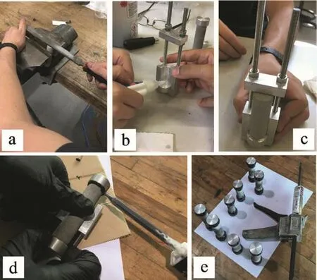
Fig. 4.The pre-processing preparation of the Mogi’s layout specimen:(a)The outer edges were smoothed initially by a fine rasp;(b)One drop of acrylic glue was applied to the end piece and the specimen interface;(c)The primary configuration was fixed via an alignment cover;(d)The structural adhesive 3M Scotch Weld was applied for the secondary gluing;and(e)The specimens remained untouched for one week.

Since the ratio between the repeatability limit and the average value of a parameter can be considered as a benchmark to measure its variability,some of the experimental data(and their ratios to the average values)obtained for the Pietra Serena sandstone by both the ASTM and Mogi’s configurations(see Table 5)are listed in Table 6.

The high variability ofE25(the ratio of testing value to the average is 0.63)of the Pietra Serena sandstone measured in this work demonstrates an undesired issue as shown by Fig. 6,where a nonlinear regime is presented at the beginning of almost all the stress-strain diagrams.Moreover,the results of experimental tests on different specimens at this regime are not the same and differ significantly.This response may have two main causes:(1)very smooth surface f i nishing on rock specimens is difficult to be obtained and the upper compressive platen therefore needs to be adjusted automatically and aligned to the surface of the specimens at the beginning of the test;and(2)the presence of the large number of pre-existence microcracks in the specimens created during their fabrication process.It is worth mentioning that the density of these microcracks is much higher near the outer edges of the specimens than that in the middle region.

We tried to reduce the effect of this phase(that is more related to specimen issue)by means of a post-processing step.For this,the linearelastic regime was determined first.Then the elastic modulusE50of each specimen was measured.The elastic regime was subsequently expanded with the same elastic modulus up to the null stress level.Finally,the whole curve was shifted along the strain axis to start of the origin.The results of the post-processing procedure are shown in Fig. 7.

The fractured specimens of the ASTM arrangement are shown in Fig. 8,exhibiting an almost identical failure mode for all the specimens.A crack initiates at the edge of the specimen and propagates mainly in the vertical direction(parallel to the axis),demonstrating that the failure mode of the ASTM configuration test is in accordance with the definition of the axial splitting failure mode as represented in Fig. 2.

2.4.Mogi’s layout experimental results

The stress-strain diagrams of the Mogi’s specimens are shown in Fig. 9.The UCSs and different extrapolations of elastic modulus for each specimen are also given in Table 5.Identical mechanical properties provided by the ASTM configuration(Table 5)can be measured for the Mogi’s arrangement,as reported in Table 6.The stress-strain diagram and the mechanical properties of specimen C3,as expressed in Fig. 9 and Table 5,respectively,show inappropriate responses.This approves the Mogi’s suggestion about the range of theL0/Dratio(L0/Dratio of specimen C3 is equal to 1.8).Therefore,the experimental data related to this specimen are not considered for computing the average values in Table 6.

The fractured specimens of the Mogi’s arrangement are shown in Fig. 10.Unlike the specimens of the ASTM configuration,shear planes are observed and the crack propagates through them.The fracture patterns of all the specimens are very similar,which is in accordance with the shearing along a single(or double)plane failure mode as represented in Fig. 2.

2.5.Comparison of the ASTM and Mogi’s configurations results

As can be seen in Table 6,the average UCS of the Mogi’s arrangement is almost equal to(or slightly higher than)the one of the ASTM standard configuration.The variability of the 25%tangent modulus,E25,of the ASTM configuration is significantly higher than that of the Mogi’s configuration,while the variability of the 50%tangent modulus,E50,is almost equal for the two layouts.The Mogi’s approach therefore prevents the undesired effects of thepre-existence microcracks close to the ends of the specimens.The Mogispecimens do not show the initial nonlinear behaviour mainly due to their larger length.The Mogi’s layout consists in longer specimens;therefore,the measurement of the displacement is less affected by the presence of the microcracks,which are concentrated near the end bases of the specimen(where the glue fillet is also presented).If the specimen is long enough,the cracks due to machining at the bases are not presented in the zone where the extensometer is applied.Therefore,the nonlinear deformation due to the presence of the cracks is notrecordedby the extensometer.In addition,the glue fillet covers partially the zone where these cracks are presented.Indeed,longer ASTM specimens(B and C series)also show lower initial nonlinear phase.Moreover,due to the utilisation of steel end pieces at the Mogi’s layout and their significant surface finishing,the upper compressive platen is almost perfectly aligned from the beginning of the test.The effects of these features are clearly visible in comparison of Fig. 11a and b,where the postprocessed stress-strain curves of the ASTM configuration exhibit an almost identical behaviour as that of the Mogi’s arrangement.

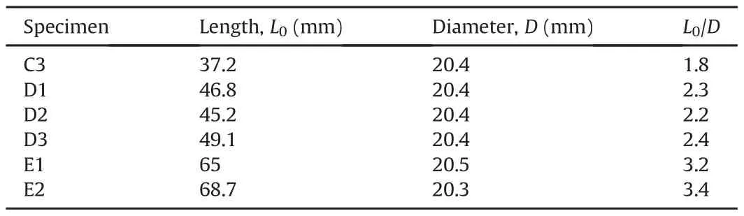
Table 3Dimensions of the specimens-Mogi’s layout.

Fig. 5.unconfined compression test apparatus-the Mogi’s configuration.

Fig. 6.The stress-strain curves of unconfined compression tests-the ASTM’s layout.

Table 4Uniaxial compressive strengths and elastic moduli for the standard configuration specimens.

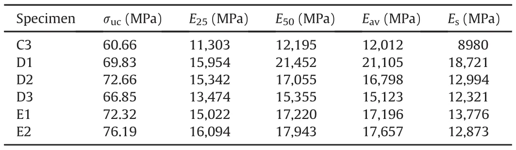
Table 5Uniaxial compressive strengths and elastic moduli for the Mogi’s specimens.

As previously discussed,the two types of specimens show different failure modes.The Mogi’s specimens have a shear failure mode(see Fig. 10),while the compressive failure mode(vertical crack propagation parallel to the loading axis)was observed for the standard arrangement(see Fig. 8).

3.Numerical modelling techniques

Many numerical modelling techniques have been developed for stress analyses of solid mechanics in the continuum domain.Among these,the conventional Lagrangian FEM offers advantages,including high accuracy and convenient time consumption cost.However,a disadvantage lies within the reduced performance of grid based numerical methods to cope with highly distorted meshes and large fragmentation,since the mesh usage for solving the problems consists of free surface,deformable boundary and moving interface,which could conduce to various struggles.

3.1.Smooth particle hydrodynamics

At present,the SPH is one of the most efficient numerical methods for dealing with continuum problem subjected to large deformations and fracture.The SPH is a “true”mesh-free method that represents the state of a system by a set of particles.These particles hold the material properties and interact in a range which is controlled by a smoothing(kernel)function.The kernel approximation for any two given particles,iandj,is determined as

wherexiandxjare the coordinates of the particles in the problem domain Ω,his the distance between the two particles,andWis the smoothing function given as follows:

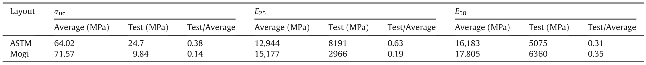
Table 6The mechanical responses of the ASTM and Mogi’s layouts under unconfined compression for Pietra Serena sandstone.

Fig. 7.The standard configuration results of unconfined compression tests after postprocessing.

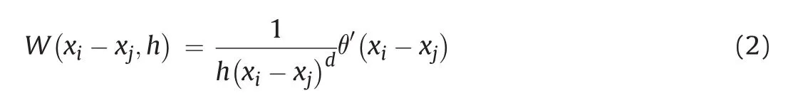
wheredis the number of space dimension,and θ′is an auxiliary function(see Fig. 12).Since the connectivity between the particles is considered as a part of the computation process,a straightforward handling of problems with extreme deformations is allowed by implementing the SPH method(Liu and Liu,2010).

3.2.Finite element method-smooth particle hydrodynamics technique

Fig. 8.The broken specimens-the ASTM configuration.

Fig. 9.The stress-strain curves of unconfined compression tests-the Mogi’s layout.

A numerical scheme,namely FEM-SPH,has been developed to account for both the FEM and SPH method.Within this numerical technique,the Lagrangian solid elements are deleted after reaching a certain criterion and are adaptively transformed to SPH particles.These SPH particles inherit exactly all of the mechanical properties of the failed mesh elements,i.e.mass,kinematic variables,and constitutive properties.

Implementation of this technique in LS-DYNA is done by calling the keyword ADAPTIVE_SOLID_TO_SPH.However,most of the material keywords available in LS-DYNA material library,i.e.the ones used in this study,do not have any internal eroding algorithm,and thus an external eroding algorithm needs to be implemented in conjunction with this keyword.The element erosion of the models used in this work was obtained using MAT_ADD_EROSION and specif i ed a certain value for the maximum effective strain at failure(EFFEPS).Therefore,each hexahedral solid element which meets this criterion is eroded,and then by defining the two input parameters of the ADAPTIVE_SOLID_TO_SPH keyword as ICPL=1 and IOPT=1,the software automatically replaces that eroded element with a certain number of SPH particles.The number of particles can be controlled by the users,i.e.it can be 1,8 or 27 in case of hexahedral elements(see Fig. 13).In this study,the failed solid elements were converted into one SPH particle to keep the time consumption low.

Fig. 10.The broken specimens-the Mogi’s configuration.

3.3.Material modelling

The material model utilised for the numerical simulation of rock specimens is called the KCC model.This KCC model,presented in the material library of LS-DYNA by MAT_CONCRETE_DAMAGE_R3(or MAT_072R3),is a material model developed by Malvar et al.(1994,1996,1997,2000).The failure function of the KCC material model can be derived by the following equation in terms of the Haigh-Westergaard stress invariants:

where ξ,ρand θare the Haigh-Westergaard coordinates;fc（ξ，ρ）corresponds to the failure surface in the triaxial compression state of stress when the Lode angleθis equal to 60?;and the dimensionless function^r［Ψ（p），θ is the ratio between the current radius of the failure surface and the compressive meridian.Eq.(3)is discussed in detail below.

The KCC model takes advantage of the three fixed independent failure surfaces in the compressive meridian(ξ-ρ plane),which correspond to the yield,ultimate and residual strengths of the material(see Fig. 14),respectively.Hence,the functionfc（ξ，ρ）is defined for each one of these failure surfaces separately as follows:

The stress invariants for an axisymmetric loading condition,when σ1= σa(the axial stress)and σ2= σ3= σl(the lateral stress),can be rewritten as

Therefore,the equations of the three failure surfaces for the axisymmetric state of stress can be respectively written as

wherepis the pressure(positive in compression),and theai-parameters are user-defined input parameters that can precisely define the failure surfaces of the KCC model.

The damage accumulation is also considered based on the current state of stress among these failure surfaces by means of a linear interpolation function.The model was described in detail in Malvar et al.(2000).An EOS is used for decoupling the volumetric and deviatoric responses.It gives the current pressure as a function of current and previous compressive volumetric strains.The EOS keyword in LS-DYNA implemented in conjunction with the KCC model is called EOS_TABULATED_COMPACTION,in which up to ten pairs of pressure-volumetric tabular data can be input to describe the rock compaction behaviour.

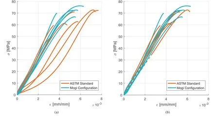
Fig. 11.Comparison of the Mogi’s configuration with(a)the original results,and(b)the post-processed results of the ASTM layout.

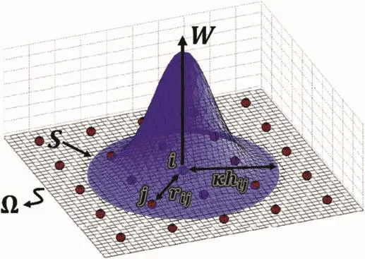
Fig. 12.SPH particles in a two-dimensional problem domain.

Two different calibration procedures are used for the numerical modelling presented in this study,which are called here as“full input mode”and “automatic mode”.The “full input mode”calibration of KCC requires 22 input parameters and another set of independent tables,which are attributed to the damage evaluation parameters(λ)corresponding to the current failure surface(η)(Hallquist,2014).However,the most significant improvement,presented in the third release of this model,provides an automatic input parameter generation opportunity for the users,based only on a few parameters,i.e.the UCS,the density and the Poisson’s ratio.Therefore,it is possible to perform a primary simulation just based on three(or even two,excluding the Poisson’s ratio)parameters,which is called in this article as the “automatic mode”.Apart from the numerical results obtained directly from the“automatic mode”,LS-DYNA also generates all the input parameters(required for the “full input mode”)automatically and writes them into the “MESSAG”file.Therefore,some of these parameters(i.e.the damage parameters)can be used in addition to other parameters that can be obtained from other resources.

The“automatic mode”of KCC model was originally developed to simulate the response of concrete,and although the response of sandstone is expected to be similar to that of concrete,the automatic input mode results are only a rough estimation for sandstones.The“automatic mode”was used initially in this study due to the overwhelming number of input parameters which are difficult to be obtained from current resources.The authors could not find any information about the mechanical response of Pietra Serena sandstone;however,an extensive literature review(Coli et al.,2002,2003,2006)revealed the presence of another rock material,called Berea sandstone,with similar mechanical properties to Pietra Serena sandstone.Berea sandstone is a sedimentary rock with high porosity and permeability,and is mostly composed of sand-sized grains(Khodja et al.,2010).Therefore,a first trial was to calibrate this material model according to the experimental data provided for Berea sandstone obtained from ASTM D7012-04(2004),as shown in Table 7.

Fig. 13.Transformed SPH particles from a hexahedral three-dimensional solid element.

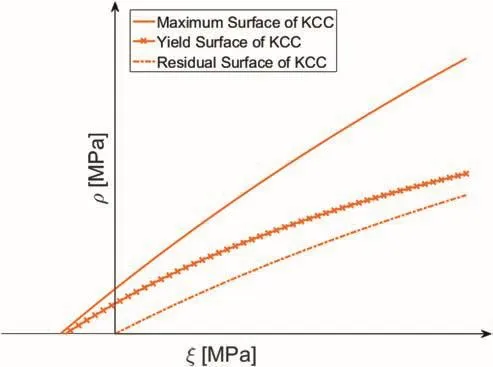
Fig. 14.The three independent failure surfaces of KCC material model in compressive meridian.

Table 7The experimental data provided for the automatic mode.

The parameters RSIZE and UCF are the unit conversion factors,and NOUT is called the “output selector for effective plastic strain”.According to Hallquist(2014),whenNOUT=2,the quantity labelled as“plastic strain”by LS-PrePost is actually the one that describes the“scaled damage measure,δ”which varies from 0 to 2.When the value ofδis still lower than one,no element(which has the KCC material model)reaches the yield limit;when the value is equal to2,the corresponding elements meet the residual failure level.It is worth mentioning that only at the automatic mode of MAT_072R3 keyword(when a maximum number of six parameters are defined),A0 should be defined as a negative value to represent the UCS.For example,-62 in Table 7 means that the UCS is equal to 62 MPa.

After performing the initial simulation,some of the generated input parameters(i.e.B1,B2,B3,ω,Sλand LOC-WIDTH)were kept constant and used at the “full input mode”(see Table 8),where the parametersB1 andB2 govern the softening in compression and uniaxial tensile strains,respectively,whereas the parameterB3 affects the triaxial tensile strain softening.The parameters ω,Sλ,Edropand LOC-WIDTH correspond to the frictional dilatancy,stretch factor,post-peak dilatancy and three times of the maximum aggregate diameter,respectively.

Almost all of the EOS tabular data were also used for the full input calibration mode.Only the “Pressure02”parameter from EOS keyword was changed to 26.1 MPa to reach the same bulk modulus(and accordingly the elastic behaviour)as the Pietra Serena sandstone.The details are described in Mardalizad et al.(2016).The tensile strength parameter was investigated in another recent study by the same authors(Mardalizad et al.,2017),where the Brazilian tensile test was performed on Pietra Serena sandstone and the tensile strength was determined as 5.81 MPa.The input parameters corresponding to the damage function,indicated by the set of η-λ data,were changed to the values reported in Markovich et al.(2011).

Table 8The results obtained from the automatic input generation mode of MAT_072R3.

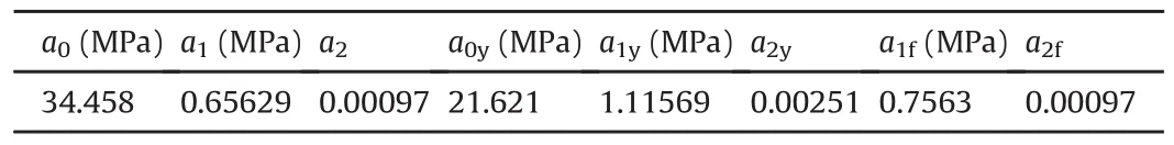
Table 9The ai-parameters provided for the full input mode.

Theai-parameters can be determined by means of the least square curve fitting method from the triaxial compression tests(Jaime,2011).The experimental data of the triaxial compression test performed at four different confining pressures were reported in Ding(2013),hence,theai-parameters are computed,as shown in Table 9.

Therefore,the specifications of the final calibrated material model are summarised in Table 10.

3.4.Replication of experimental tests

Two numerical models were developed in LS-DYNA to replicate the unconfined compression tests in both the ASTM and the Mogi configurations(see Fig. 15).All the geometry parts were generated,assembled and meshed by ABAQUS explicit software and then imported in LS-PrePost to specify the required keywords.The mesh convergence studies were performed based on the elements’sizes of the specimens,and 1 mm was considered for these elements.The mesh sizes of the other components were determined by considering the requirements of the contact treatments,i.e.the element size of the slave parts was considered lower than that of the master ones.The numerical models of rocks in the replicated ASTM and Mogi’s configurations have the same geometries with the specimens of classes C and D,respectively.

Fig. 15.Numerical models developed in LS-DYNA to replicate(a)the ASTM configuration,and(b)the Mogi’s configuration.

Fig. 16.Comparison of the kinetic energy-time and internal energy-time diagrams of(a)the ASTM configuration,and(b)the Mogi’s configuration.

Table 11Material keywords and their corresponding mechanical properties for both the ASTM and Mogi models.

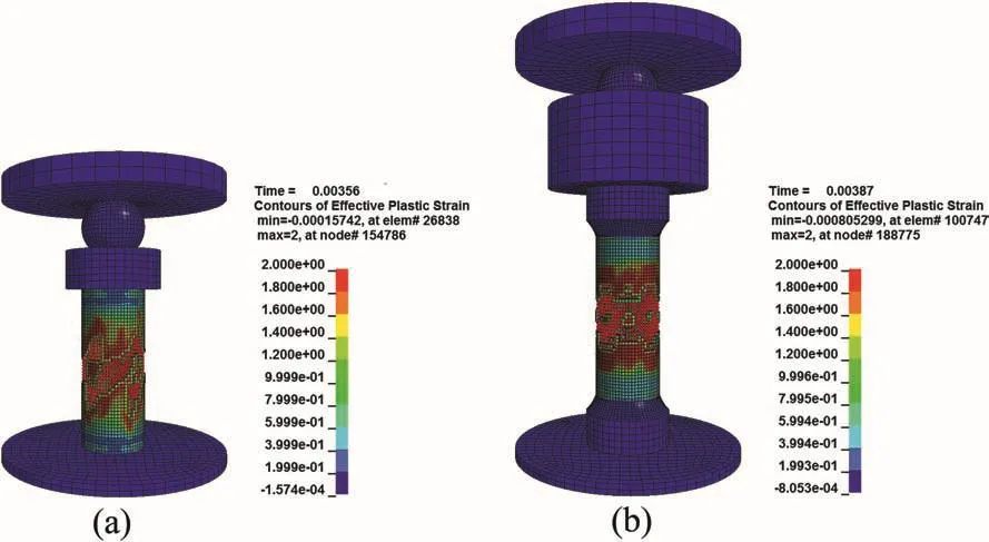
Fig. 17.Distribution of the scaled damage parameter after failure:(a)the ASTM configuration,and(b)the Mogi’s configuration(unit:ms).

The numerical model of the ASTM configuration consists of five parts including two rigid platens(representing the compressive platens),one elastic sphere,one elastic cylinder(representing the spherical seat),and the specimen.The displacement-controlled compression loading was imposed by the upper platen and the lower platen was fixed(zero degree of freedom).The numerical model of the Mogi’s configuration consists of nine parts,five of them identical to those of the ASTM configuration,plus two aluminium cylinders and two round profiles(representing the profile of the epoxy).Displacement-controlled loading is applied to the upper compressive platen(for both models)at a rate of 0.45 mm/ms,and the simulations are terminated after 5 ms.This loading rate(0.45 mm/ms)has been considered since it is more convenient to reduce the computation cost in the quasi-static analyses by the time-scaling approach.However,in this case,the kinetic energy should be monitored to ensure that the ratio of kinetic energy to internal energy does not become too large(typically less than 10%).Fig. 16 shows the diagrams of kinetic energy-time and internal energy-time of both the ASTM and Mogi’s configurations.As can be seen,the amount of kinetic energy in both cases is negligible(less than 1%);therefore,it suggests that the loading rate is acceptable.

Fig. 18.Magnified distribution of the scaled damage parameter after failure:(a)the ASTM configuration,and(b)the Mogi’s configuration.

The material keywords and their corresponding mechanical properties for both models are reported in Table 11.The combination of CMO,CON1 and CON2 expressed in Table 11 determines the degree of freedom of a rigid body in LS-DYNA.The rigid body considered for the upper compressive platen has only one translational degree of freedom inz-direction,while the lower compressive platen has no degree of freedom.

The hexagonal solid elements,with constant stress element formulation,were implemented for all the FEM’s geometry parts.The SPH section was set by the default values of LS-DYNA.The automatic penalty based contact was applied to both the solid solid and the SPH-solid contacts.The static friction coefficient was equal to 0.4 for all the contact keywords containing the rock specimen(as their slave segments).The static friction coefficient of the contact between the spherical seated cylinder and the upper aluminium end piece of the Mogi’s configuration was set to 0.45.Since the seating sphere was covered by grease during the experimental tests,the static friction coefficients of all the contact keywords containing this sphere were set to 0.05.However,the constraint-based contact was considered as the contact treatment between the sections related to the epoxy pro fi le.

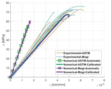
Fig. 20.Comparison of experimental data and numerical results.

The adaptive conversion of mesh elements to the SPH particles was applied only to the specimens.The EFFEPS,which is considered as the conversion limit,should be defined as the final step for the numerical simulation.For this purpose,the simulation should be fi rst run without the MAD_ADD_EROSION implementation to examine the presence of highly distorted elements and to identify the EFFEPS at that time step.In this study,the EFFEPS was set to 0.03.

3.5.Numerical results

In order to obtain the numerical stress-strain diagram,the stress was calculated from the reaction force between the platens and the specimen.The axial strain was computed starting from the axial displacements measured at 8 mm and 20 mm length spans(in the middle cross-section of the specimens)for the ASTM and Mogi’s configurations,respectively(similar to the gauge lengths of their extensometers).The distributions of scaled damage measure,δ,of the calibrated(full input)model for both the ASTM and Mogi’s configurations are captured at one time step after failure and indicated in Fig. 17 to express the crack propagation patterns.

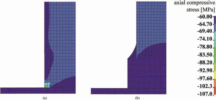
Fig. 19.The distribution of the axial compressive stress of(a)the ASTM configuration,and(b)the Mogi’s configuration.

Table 12Comparison of the UCS values obtained by numerical simulation and experiments.

Table 13Comparison of E50values obtained by numerical simulation and experiments.

The SPH particles which are in charge of dealing with severe deformation in Fig. 17 represent the crack propagation pattern.The critical parts of the specimens in Fig. 17 are Magnified in Fig. 18 to indicate more clearly the crack pattern.As can be seen in Fig. 18a,the numerical model results of the replicated ASTM configuration do notdemonstrateanyordered crack pattern.This failure is caused by the lack of nodes at either the top or bottom of the specimens fixed in tangential direction.This is one of the conditions that yield disordered crack patterns described in detail in Murray et al.(2007).However,the presence of some vertical cracks can be considered as an acceptable agreement with the crack propagation pattern obtained by the experimental tests.

As can be seen in Fig. 18b,a series of X-pattern cracks follows the double diagonal damage bands,which proves the presence of shear failure planes.Therefore,the failure of the Mogi’s configuration model represents the double-shear failure mode in Fig. 2.Although this is not the same as the failure mode obtained from the experimental tests(i.e.shearing along single plane failure),the divergence can be justi fi ed based on the(ideal)symmetrical condition,e.g.loading,contact interfaces,and boundary conditions,exerted by numerical modelling.It has been tried to overthrow the full symmetry of the system,but it neither changed the failure mode,nor achieved stable results.Therefore,the precise failure mode obtained from the experimental tests cannot be reproduced by this numerical simulation technique.

The stress distributions along the axial direction(compressive stress)for both the ASTM and the Mogi’s configurations are expressed in Fig. 19.The presence of the stress concentration at the outer edge of the specimen,which was expected based on the research of Mogi(2007),is visible in the ASTM model.However,the Mogi’s model exhibits a more uniform stress distribution.

Fig. 21.The numerical stress-strain diagrams of the ASTM model in(a)the automatic mode,and(b)the full calibration mode.

Fig. 22.The numerical stress-strain diagrams of the Mogi model in(a)the automatic mode,and(b)full calibration mode.

4.Comparison of experimental and numerical results

The stress-strain diagrams of the KCC models(both the ASTM and the Mogi models)in the automatic input generation mode and the full input calibration mode are compared to the experimental results,as shown in Fig. 20 and Tables 12 and 13.As expected,the results obtained by the automatic input mode are not in agreement with the experimental data.This is more critical in the elastic regime,in which the numerical model overestimates the average Young’s modulus by more than twice the values obtained experimentally(see Figs.21 and 22).However,the ultimate failure level can be acceptable.This rough response of the KCC model in its automatic mode indicates the different behaviours of concrete(to which the model is addressed)compared with sandstone,especially in the elastic regime.The numerical results obtained by the fully calibrated mode of KCC model,on the other hand,show significant agreement with the experimental data.Therefore,it can be concluded that the KCC is an efficient material model for numerical simulation of the rock materials,in particular for sandstones.

5.Conclusions

Experimental tests were performed based on the protocols of the ASTM standard and on the Mogi’s enhancement configuration.The average experimental UCS of Pietra Serena sandstone was measured as 67 MPa.The results of Mogi and ASTM configurations are comparable,and it shows that the Mogi’s configuration reduces the variability of results and the sensitivity to the specimen geometrical deviations.

A numerical model using the FEM in conjunction with the SPH was implemented using the KCC material model.The KCC model shows a significant improvement when the material input parameters are calibrated and directly inserted into the material keyword,instead of the automatic input generator mode.The specifications of the calibrated material model are summarised in Table 10.

The numerical model developed by the KCC automatic input mode underestimates the UCS by 16.6%and overestimates the elastic modulus by104.5%,while these values significantly decrease to 6.1%and 21.3%,respectively,after implementing the calibrated input mode.

The coupling SPH and FEM technique is proved to be a reliable method to simulate crack generation.The numerical results are still expected to be improved by a direct material identification based on the Pietra Serena sandstone,i.e.the triaxial compression and isotropic compression tests.However,the numerical simulations in this study prove the functionality and reliability of the KCC material model in the replication of the unconfined compression test.

Conflict of interest

The authors wish to confirm that there are no known Conflicts of interest associated with this publication and there has been no significant financial support for this work that could have influenced its outcome.

Åkesson U,Hansson J,Stigh J.Characterisation of microcracks in the Bohus granite,western Sweden,caused by uniaxial cyclic loading.Engineering Geology 2004;72(1-2):131-42.

Anghileri M,Castelletti LML,Francesconi E,Milanese A,Pittofrati M.Rigid body water impact-experimental tests and numerical simulations using the SPH method.International Journal of Impact Engineering 2011;38(4):141-51.

ASTM D7012-04.Standard test method for compressive strength and elastic moduli of intact rock core specimens under varying states of stress and temperatures.West Conshohocken,USA:ASTM International;2004.

Attewell P,Farmer I.Principles of engineering geology.London:Chapman and Hall;1976.

Basu A,Celestino TB,Bortolucci AA.Evaluation of rock mechanical behaviors under uniaxial compression with reference to assessed weathering grades.Rock Mechanics and Rock Engineering 2009;42(1):73-93.

Basu A,Mishra D,Roychowdhury K.Rock failure modes under uniaxial compression,Brazilian,and point load tests.Bulletin of Engineering Geology and the Environment 2013;72(3-4):457-75.

Bieniawski ZT.Rock mechanics design in mining and tunnelling.Rotterdam:A.A.Balkema;1984.

Brace WF,Paulding BW,Scholz C.Dilatancy in the fracture of crystalline rocks.Journal of Geophysical Research 1966;71(16):3939-53.

Brady BH,Brown ET.Rock mechanics:for underground mining.Springer;2013.

Bresciani L,Manes A,Romano T,Iavarone P,Giglio M.Numerical modelling to reproduce fragmentation of a tungsten heavy alloy projectile impacting a ceramic tile:adaptive solid mesh to the SPH technique and the cohesive law.International Journal of Impact Engineering 2016;87:3-13.

Ceryan N,Okkan U,Kesimal A.Prediction of unconfined compressive strength of carbonate rocks using artif i cial neural networks.Environmental Earth Sciences 2013;68(3):807-19.

Coli M,Livi E,Tanini C.Pietra Serena mining in Fiesole.Part I:historical,cultural,and cognitive aspects.Journal of Mining Science 2002;38(3):251-5.

Coli M,Livi E,Pandeli E,Tanini C.Pietra Serena mining in Fiesole.Part II:geological situation.Journal of Mining Science 2003;39(1):56-63.

Coli M,Livi E,Tanini C.Pietra Serena mining in Fiesole.Part III:structural-mechanical characterization and mining.Journal of Mining Science 2006;42(1):74-84.

Ding J.Experimental study on rock deformation and permeability variation.MS Thesis.Texas A&M University;2013.

Eni.Enciclopedia degli idrocarburi.Roma,Italy:Istituto Della Enciclopedia Italiana Fondata Da Giovanni Treccani S.p.a.;2007(in Italian).

Hallquist JO.LS-DYNA® keyword user’s manual,volumes I-III(LS-DYNA R7.1).Livermore,USA:Livermore Software Technology Corporation(LSTC);2014.

Hudson JA,Harrison JP.Engineering rock mechanics:an introduction to the principles.Elsevier;2000.

Jaeger JC,Cook NGW,Zimmerman RW.Fundamentals of rock mechanics.4th ed.John Wiley&Sons,Inc.;2007.

Jaime MC.Numerical modeling of rock cutting and its associated fragmentation process using the finite element method.PhD Thesis.University of Pittsburgh;2011.

Kahraman S.Evaluation of simple methods for assessing the uniaxial compressive strength of rock.International Journal of Rock Mechanics and Mining Sciences 2001;38(7):981-94.

Khodja M,Khodja-Saber M,Canselier JP,Cohaut N,Bergaya N.Drilling fluid technology:performances and environmental considerations.In:Fuerstner I,editor.Products and services;from R&D to final solutions.Sciyo;2010.p.227-56.

Kochavi E,Kivity Y,Anteby I,Sadot O,Ben-Dor G.Numerical model of composite concrete walls.In:Proceedings of the ASME 2008 9th Biennial conference on engineering systems design and analysis(ESDA2008).American Society of Mechanical Engineers(ASME);2009.

Lacy WC,Lacy JC.History of mining.In:Hartman HL,editor.SME mining engineering handbook.2nd ed.Society for Mining,Metallurgy,and Exploration Inc.;1992.p.5-23.

Li L,Lee PKK,Tsui Y,Tham LG,Tang CA.Failure process of granite.International Journal of Geomechanics 2003;3(1):84-98.

Liu M,Liu GR.Smoothed particle hydrodynamics(SPH):an overview and recent developments.Archives of Computational Methods in Engineering 2010;17(1):25-76.

Malvar LJ,Crawford JE.Dynamic increase factors for concrete.Naval Facilities Engineering Service Center;1998.

Malvar LJ,Crawford JE,Wesevich JW,Simons D.A new concrete material model for DYNA3D.1994.

Malvar L,Crawford J,Wesevich J,Simons D.A new concrete material model for DYNA3D-release II:shear dilation and directional rate enhancements.Report TR-96-2.2.Defense Nuclear Agency;1996.

Malvar LJ,Crawford JE,Wesevich JW,Simons D.A plasticity concrete material model for DYNA3D.International Journal of Impact Engineering 1997;19(9-10):847-73.Malvar LJ,Crawford JE,Morrill KB.K&C concrete material model release III-automated generation of material model input.K&C Technical Report TR-99-24-B1;2000.

Mardalizad A,Manes A,Giglio M.An investigation in constitutive models for damage simulation of rock material.Associazione Italiana per L’Analisi delle Sollecitazioni(AIAS),Università degli studi di Trieste;2016.

Mardalizad A,Manes A,Giglio M.Investigating the tensile fracture behavior of a middle strength rock:experimental tests and numerical models.In:The 14th international conference on fracture(ICF14);2017.Rhodes,Greece.

Markovich N,Kochavi E,Ben-Dor G.An improved calibration of the concrete damage model.Finite Elements in Analysis and Design 2011;47(11):1280-90.

Martin CD.The strength of massive Lac du Bonnet granite around underground openings.PhD Thesis.Winnipeg,Canada:University of Manitoba;1993.

Mogi K.Some precise measurements of fracture strength of rocks under uniform compressive stress.Rock Mechanics and Engineering Geology 1966;4(4):41-55.

Mogi K.Experimental rock mechanics.CRC Press;2007.

Murray YD,Abu-Odeh AY,Bligh RP.Evaluation of LS-DYNA concrete material model 159.Report No.FHWA-HRT-05-063.Federal Highway Administration;2007.

Nazir R,Momeni E,Armaghani DJ,Amin MM.Correlation between unconfined compressive strength and indirect tensile strength of limestone rock samples.Electronic Journal of Geotechnical Engineering 2013;18:1737-46.

Olleak AA,El-Hofy HA.SPH modelling of cutting forces while turning of Ti6Al4V alloy.In:Proceedings of the 10th European LS-DYNA conference.DYNAmore GmbH;2015.

Pepper JF.Geology of the Bedford shale and Berea sandstone in the Appalachian basin:a study of the stratigraphy,sedimentation and paleogeography of rocks of Bedford and Berea age in Ohio and adjacent states.US Government Printing office;1954.

Santarelli FJ,Brown ET.Failure of three sedimentary rocks in triaxial and hollow cylinder compression tests.International Journal of Rock Mechanics and Mining Sciences&Geomechanics Abstracts 1989;26(5):401-13.

Szwedzicki T.A hypothesis on modes of failure of rock samples tested in uniaxial compression.Rock Mechanics and Rock Engineering 2007;40(1):97-104.

Wu Y,Crawford JE.Numerical modeling of concrete using a partially associative plasticity model.Journal of Engineering Mechanics 2015;141(12).https://doi.org/10.1061/(ASCE)EM.1943-7889.0000952.04015051.

Zhao H,Zhang C,Cao WG,Zhao MH.Statistical meso-damage model for quasibrittle rocks to account for damage tolerance principle.Environmental Earth Sciences 2016;862:75.https://doi.org/10.1007/s12665-016-5681-7.