Analysis of a System Describing Proliferative-Quiescent Cell Dynamics∗

Jean CLAIRAMBAULTBenoît PERTHAMEAndrada Quillas MARAN

(Dedicated to Philippe G.Ciarlet on the occasion of his 80th birthday)

1 Introduction

Systems describing the dynamics of proliferative and quiescent cells are commonly used as computational models,for instance for tumor growth and hematopoiesis(see[4,10,14—16,23]).The typical dynamical system,introduced in the papers of Gyllenberg and Webb[13],describes the populations nP(t)≥0(proliferative cells)and nQ(t)≥0(quiescent cells)with a control by the total population n(t),as

Here,β＞ 0 represents the cumulated proliferation rate of proliferative cells,δ＞ 0 represents the death rate of quiescent cells,the smooth function s+＞ 0,s−≥ 0 define controls of the system.The authors in[13]showed the nonlinear stability of the non-zero steady state using the Poincar´e-Bendixson theorem.

Our purpose is to introduce another argument,based on an energy functional,or Lyapunov functional in the language of dynamical systems,which leads to an analytical method that can be extended to more elaborated models.We have in mind two extensions.

Firstly,we consider partial differential systems which take into account spatial extension and random motion of cells.Consider a smooth and bounded region Ω of Rd,the simplest system is

with smooth initial data nP(x)＞0,(x)＞0.Again our purpose is to study the long term convergence in this case,using our energy functional.

Secondly,we have in mind to introduce more complex biological content.This is the case in hematopoiesis where the dynamic(1.1)represents a two stage stem cell population.We may add a third compartment which corresponds to the early progenitor cells encountered in hematopoiesis,and written as

Figure 1 Diagram of the three compartmental model(1.2).

Here nP(t)and nQ(t)stand for a population of proliferative and quiescent stem cells,respectively,while u(t)represents the corresponding population of early progenitor cells,assumed to proceed from proliferative stem cells only.Note that we allow a fraction η of progenitor cells to de-differentiate and go back to the proliferative stem cell compartment,a case that in principle occurs only in cancer(in particular leukemic)cell populations(see[3]).In this representation,we do not consider the whole hematopoietic tree(as done in,e.g.,[2,24]),but only its most immature components.Indeed,having in mind,as in[2,24],future applications to acute myeloid leukemia,that emerges from these early stages(see[17]),we believe that this is the right place in the hematopoietic tree to set the relevant mathematical model and its analysis.

The rest of the paper is organized as follows.In Section 2,we introduce the assumptions and the energy method and we use it for the system(1.1)in order to prove its global,nonlinear asymptotic stability.In Section 3,we analyze the PDE system(3.1)and show that the energy functional can be used to prove again the long time convergence to the homogeneous steady state.The last section is devoted to the construction of a variant of the energy functional adapted to the three-compartment system(1.2).

2 Assumptions and the Energy Method

2.1 Assumptions and convergence to the non-zero steady state

Following[13],we consider that the parameters satisfy the following assumptions.

Assumptions for the existence of a unique non-zero steady state

Assumption for global stability

With the assumptions(2.1)—(2.2),it is well established(see[13])that there is a unique non-zero steady state of system(1.1)which is characterized by

Additionally,with the assumption(2.3),one can prove that,as t→∞,

2.2 The energy method

For convenience,we change the variables and the time of the system to

Nonetheless,in what follows we still denote the time by t.In these new variables,the system reads

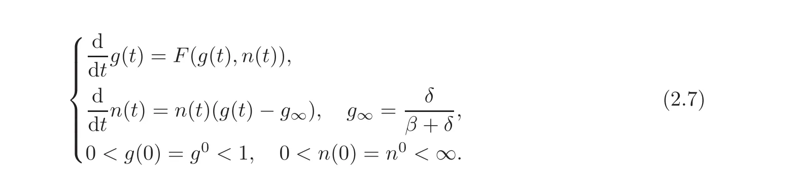
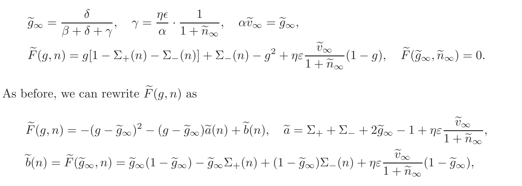
The nonlinearity is defined as F(g,n)= −g2+g[1−Σ+(n)−Σ−(n)]+Σ−(n),which we also write as

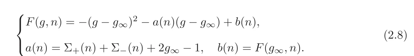
With these notations and the assumptions(2.1)—(2.3),we obtain that a(·),b(·)are smooth and bounded functions.The properties of a(·),b(·),and the definition of the steady state n∞,can be written as

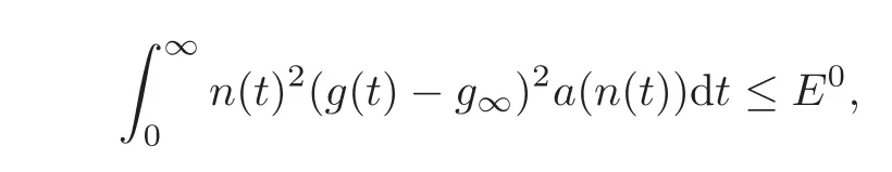
We introduce the energy of the system

with,using assumption(2.9),

Lemma 2.1With the assumptions(2.9)–(2.10),the energyE(t)defined by(2.11)is decreasing and,for(g0,n0)/=(g∞,n∞),we have

ProofWe compute

Then we conclude using the definition of a(·)in(2.8).

2.3 The convergence theorem

We are now ready for our version of the convergence result in[13],

Theorem 2.1With the assumptions(2.9)–(2.10),the solutions of(2.7)are bounded and,ast→∞,g(t)→g∞andn(t)→ n∞.

Proof(i)Because of the energy inequality(2.13),we have E(t)≤E(0)and thus G(n(t))≤E(0).We conclude that n(t)is bounded using(2.12).

(ii)Because n and g are bounded,the equation(2.7)shows that n and g are Lipschitz continuous.Therefore,n(·)2(g(·)− g∞)2is also bounded and Lipschitz continuous.Since from the energy dissipation we have

we conclude that,as t→∞,we have

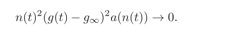
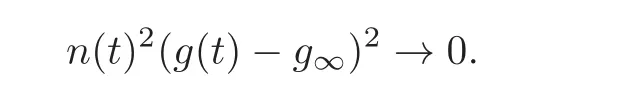
Because of assumption(2.10),this implies that

(iii)Because the energy decays,it has a limit E∞.Combined with the above information,we conclude that,as t→∞,we have

and by continuity n(t)has a limit.

(iv)Arguing by contradiction,we assume that=0.Then,for t large enough,the dynamics of g(t)resembles the solution of the Riccati equation

As t→ ∞,the solution g(t)of this equation tends tog∞.This last inequality holds thanks to the assumptions(2.9)—(2.10).But inserting this information in the equation for n(t)shows that n(t)→∞which is impossible,this is a contradiction.Therefore/=0.

(v)As a consequence,from step(ii)we deduce that g(t)→ g∞.From the equation for g(t),we conclude that b=0 which means that=n∞.

3 Model with Space and Diffusion

The method with the energy/Lyapunov functional presents another advantage which is a possible extension to the context where spatial distribution is also considered.An example is the case with spatial diffusion and we now consider distributions nP(x,t),nQ(x,t)with x ∈ Ωa smooth bounded domain of Rd.We use the equations:

This system is completed with smooth initial data(x)＞0,(x)＞0.It is of semi-linear type and global existence is granted because the nonlinearity is Lipschitzian,and solutions are smooth and positive(see[6,11,20,22]).Solutions are only locally bounded with possibly exponential growth.

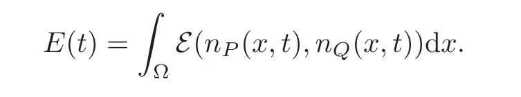
In order to adapt the energy functional E(t)defined by(2.11)to the case at hand,we need to go back to the unknowns nP,nQand use

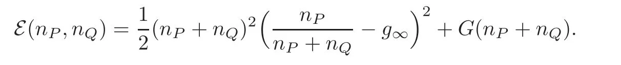
We now define the total energy with

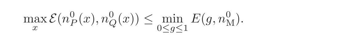
We may now state our result for the system with space.It is of global nature but with a restriction on the initial data which is limited by the convexity region of the energy .

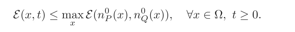
Theorem 3.1We make the assumptions(2.1)–(2.3)and thatenough(less thann∞is enough).Then,there is a smooth solution to the semi-linear parabolic system(3.1)and it satisfiesn(x,t)≤,the total energyE(t)decays and,ast→ ∞,

The end of the section is devoted to prove this theorem.

3.1 Convexity of

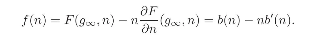
To begin with,we need to study the convexity properties of .For that purpose,we define a function which is essential for our study

We may calculate the Hessian of

still with n=nP+nQ,g=.We can compute

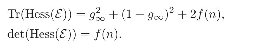
Because convexity is equivalent to the non-negativity of these two quantities,it is reduced to those n such that f(n)≥ 0.Clearly this is the case for n ≤ n∞since F(g∞,·)is positive on this interval and decreasing(see assumptions(2.9)—(2.10)).

However,we can see that for n large,this condition cannot be fulfilled.Indeed,f(n) ≥ 0 means b(n)−nb′(n)≥ 0,which would imply that b(n)=F(g∞,n)→ −∞ as n → ∞ while we assume that F is bounded.

3.2 Condition on the initial data

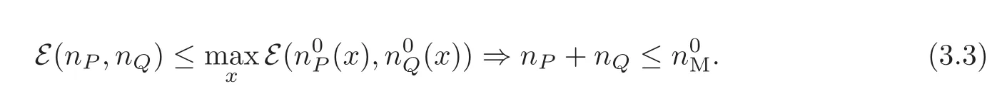
When the Laplacian is considered,it is useful to preserve the convexity zone all along the dynamics(see e.g.[6,11,20,22]).Therefore,we need a condition on the initial data which we state as follows.Consider the valuenecessarily larger than n∞,such that

We assume that

This somehow abstract condition can be satisfied with more explicit assumptions,for instance

This is the precise size condition needed in the statement on Theorem 3.1.

3.3 Conclusion

We may now conclude the proof of this theorem which relies on very standard tools for parabolic systems.Therefore,we just indicate the reason why assumption(3.2)is used.We compute the energy dissipation relation

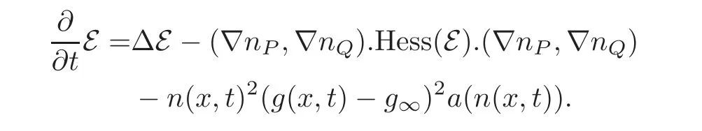
Because initially we have Hess( (t=0,x))≤ 0 for all x ∈ Ω,we conclude from the maximum principle that

Therefore the condition(3.3)tells us that n(x,t) ≤and the definition(3.2)implies that (t,x)remains convex all along the dynamics.Therefore the solution satisfies

Standard use of the energy dissipation leads to the conclusion that(∇nP(x,t),∇nQ(x,t))belongs to L2(R+;Ω).Time compactness follows from the Lions-Aubin Lemma,and thus the family(∇nP(x,t),∇nQ(x,t))converges,as t→ ∞ to an homogeneous state for large times.Finally,the reasoning of Subsection 2.3 leads to the conclusion of Theorem 3.1.

4 The 3-Compartment Hematopoiesis System

Theflexibility of the energy method for the model with proliferative and quiescent cells can also be illustrated with a 3 by 3 system.This type of model is used for describing hematopoietic stem cell dynamic and a third compartment corresponds to the early progenitor cells encountered in hematopoiesis which are denoted by u(t)in this section.Hematopoiesis is a wide subject,with several mathematical faces and the interested reader can consult for instance[1,9,21].

4.1 The model equation

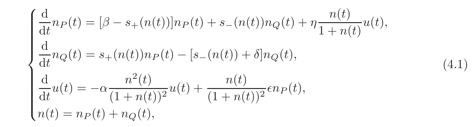
The system proposed here is the extension of(1.1)written as

where we still use the notations and assumptions of Section 2.We consider that the exchanges between the proliferating hematopoietic stem cells and the early progenitor compartment are small,i.e.,we are going to consider the perturbative regime

We assume here that de-differentiation of the progenitor cells into hematopoietic stem cells(the passage from u to nPmeasured by η)is much less important than the maturation of hematopoietic stem cells(the converse passage).De-differentiation has been observed in recent biological studies on cancers(see[5,12,25]),and investigated in modelling studies by varying its rate(see[3,18]).However,nothing is known for certain concerning its actual rate in different types and stages of cancers,nor whether it is cause or consequence of cancer emergence,except the fact that high de-differentiation rates seem to be related to cancer aggressiveness.The case η≪ε is thus relevant,at least in health or in very early cancer initiation.

However a difficulty remains;the energy dissipation −n2a(n)(g− g∞)in(2.13)does not provide enough coercivity by lack of a term n− n∞.For that technical reason,we have introduced a modulation of the exchanges with the ratioand the energy modulation has to be tuned appropriately.

We notice that solutions exist globally because positivity is preserved and the total number of cells is controlled by

and the Gronwall lemma controls the solutions with an exponential growth in time.

We perform the same change in unknowns(see equations in(2.6))as in Section 2.Set u=εv,and we get

with the following definitions,in particular of the steady state

and the assumptions(2.1)—(2.3)have to be reinforced so as to yield the positivity ofand the property0,＜ 0,then there are a0and∞such that

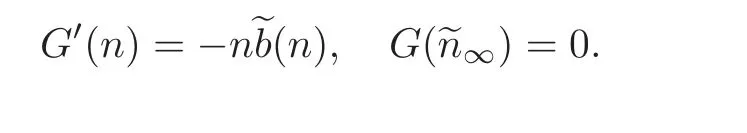
We also define G(·)with

4.2 The energy functional and long-term convergence

We need to introduce a modulation of the energy functional E(t)in order to take into account the third component.Now,we define the energy by

where the constant λ is positive and small.

Theorem 4.1Forλ ＞ 0small enough compared toα,a0andb(·),andηεsmall enough,we have,for somep∈(0,1),

Therefore,we have the long term convergence

In this theorem,the only new difficulty relies on the elaboration of the energy dissipation.The convergence result then follows exactly as in Section 2 and we skip its proof.In the end of this section,we concentrate on the dissipation of energy.

4.3 Proof of Theorem 4.1

We may compute

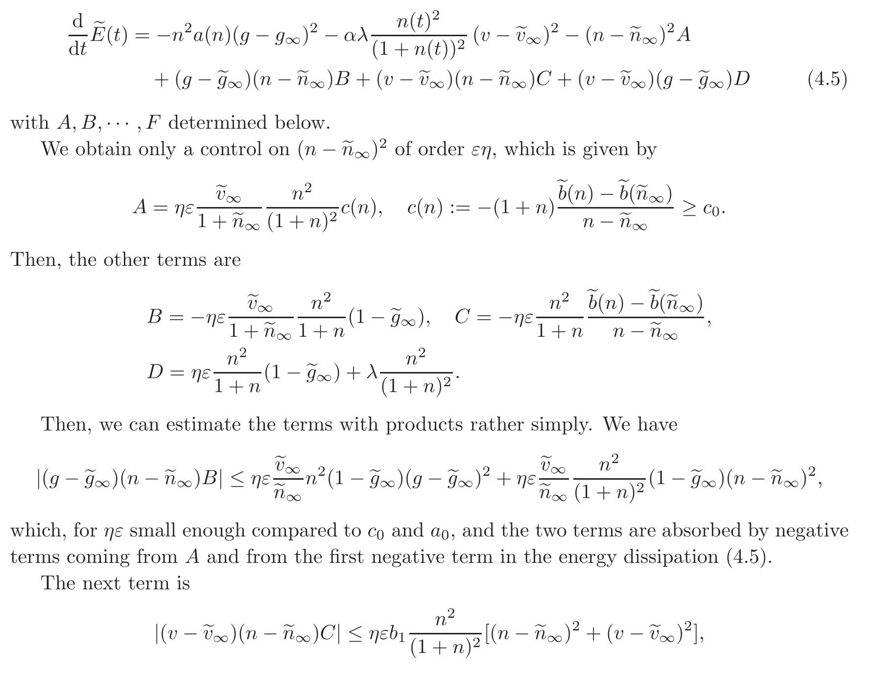
which again,for ηε small enough compared to c0,α andcontribution is absorbed by the negative terms.Here we have used

4.4 Simulations

We illustrate the behaviour of the 3∗3 system(4.1)with some numerical simulations.We have used the parameters

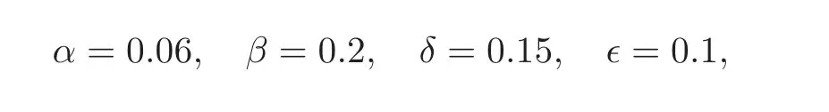
and the functions

Figure 2 displays the solution with three values of the de-differentiation parameter η,

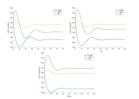
Figure 2 Numerical solution of the 3 ∗ 3 system(4.1)with three values of the de-differentiation parameter.Left:η=0.Center:η=0.01.Right:η=0.05.

5 Conclusion and Perspectives

In this study,we have considered a new method,of the energy/Lyapunov type,to analyze the asymptotic behavior of a stem/progenitor cell population model representing the very early stages of cell lineage maturation in health and cancer.Knowing the very low level of division in stem cells(as low as once a year for hematopoietic stem cells,as measured in[7—8]),it has appeared relevant since the studies of Gyllenberg and Webb[13](and earlier,of Mackey and followers[19],using age-structured models)to represent the stem cell population as compartmentalized between proliferative(cells that are engaged in the division cycle)and quiescent cells(those that are not).We have adpted this point of view here as well,with the adjunction of another maturation state,early progenitor cells,for which,for the sake of simplicity,we do not distinguish between proliferative and quiescent states.

Taking advantage of recent biological observations(see[5,12,25]),we have introduced the possibility of de-differentiation from this early progenitor state to stem cell state.As briefly sketched in the text,not much is known about the actual rate of de-differentiation in health and disease,except that it has been observed at high levels in aggressive cancers.We have assumed in our proofs low levels of this rate,meaning that its rigorous relevance may be limited to health settings or initiating cancers.Nevertheless,numerical studies in other modelling contexts(see[3,18])have shown that increasing its level increases the severity of the cancer at stake,and its evolution towards insensitivity to therapy,i.e.,drug resistance.

Last but not least,the method we have developed in this analytical study,of the energy/Lyapunov type,allowed us to extend previous studies,initiated by Gyllenberg and Webb(see[13]),who took advantage of the Poincar´e-Bendixson theorem for plane analysis,to higherdimensional analysis on the one hand,and to a 2-dimensional spatial model with diffusion on the other hand.We believe that both these extensions open new directions of research in the study of proliferative-quiescent cell population models.

AcknowledgementsThe authors gratefully acknowledge the expert contribution to this work of Fran¸cois Delhommeau and Pierre Hirsch by frequent and long tutorial discussions they led with us about normal human hematopoiesis and early leukemogenesis in the department of hematology at Hospital St Antoine in Paris.

[1]Adimy,M.and Crauste,F.,Mathematical model of hematopoiesis dynamics with growth factordependent apoptosis and proliferation regulations,Math.Comput.Modelling,49(11–12),2009,2128–2137.

[2]Adimy,M.,Crauste,F.and Abdllaoui,A.E.,Discrete maturity-structured model of cell differentiation with applications to acute myelogenous leukemia,Journal of Biological Systems,16(3),2008,395–424.

[3]Alexandra,J.and Ryan,N.G.,Effect of Dedifferentiation on Time to Mutation Acquisition in Stem Cell-Driven Cancers,PLoS Computational Biology,10(3),2014,https://doi.org/10.1371/journal.pcbi.1003481.

[4]Bresch,D.,Colin,T.,Grenier,E.,et al.,Computational modeling of solid tumor growth:The avascular stage,SIAM J.Sci.Comput.,32(4),2010,2321–2344.

[5]Cai,S.,Fu,X.,and Sheng,Z.,Dedifferentiation:A new approach in stem cell research,AIBS Bulletin,57(8),2007,655–662.

[6]DiBenedetto,E.,Partial Differential Equations,Cornerstones,2nd edition,Birkhäuser,Boston,2010.

[7]Dingli,D.and Pacheco,J.M.,Allometric scaling of the active hematopoietic stem cell pool across mammals,PLoS One,1(1),2006,https://doi.org/10.1371/journal.phone.0000002.

[8]Dingli,D.,Traulsen,A.and Pacheco,J.M.,Compartmental architecture and dynamics of hematopoiesis.PLoS One,2(4),2007,https://doi.org/10.1371/journal.phone.0000345.

[9]Drobnjak,I.,Fowler,A.C.and Mackey,M.C.,Oscillations in a maturation model of blood cell production,SIAM J.Appl.Math.,66(6),2006,2027–2048.

[10]Dyson,J.,Villella-Bressan,R.and Webb,G.,A maturity structured model of a population of proliferating and quiescent cells,Arch.Control Sci.,9(45)(1–2),1999,201–225.

[11]Evans,L.C.,Partial differential equations,Graduate Studies in Mathematics,19,American Mathematical Society,Providence,RI,2010.

[12]Friedmann-Morvinski,D.and Verma,I.M.,Dedifferentiation and reprogramming:Origins of cancer stem cells,EMBO Reports,15,2014,244–253.

[13]Gyllenberg,M.and Webb,G.F.,Quiescence as an explanation of gompertzian tumor growth,Growth,Development,and Aging:GDA,53(1–2),1989,25–33.

[14]Gyllenberg,M.and Webb,G.F.,A nonlinear structured population model of tumor growth with quiescence,J.Math.Biol.,28(6),1990,671–694.

[15]Gyllenberg,M.and Webb,G.F.,Quiescence in structured population dynamics:Applications to tumor growth,Mathematical Population Dynamics(New Brunswick,NJ,1989),Lecture Notes in Pure and Appl.Math.,131,Dekker,New York,1991,45–62.

[16]Hartung,N.,Parameter non-identifiability of the Gyllenberg-Webb ODE model,J.Math.Biol.,68(1–2),2014,41–55.

[17]Hirsch,P.,Zhang,Y.,Tang,R.,et al.,Genetic hierarchy and temporal variegation in the clonal history of acute myeloid leukaemia,Nature Communications,7(12475),2016,DOI:10.1038/ncomms12475.

[18]Leder,K.,Holland,E.C.and Michor,F.,The therapeutic implications of plasticity of the cancer stem cell phenotype.PLoS One,5(12),2010,https://doi.org/10.1371/journal.phone.0014366.

[19]Mackey,M.C.,Unified hypothesis for the origin of aplastic anemia and periodic hematopoiesis,Blood,51(5),1978,941–956.

[20]Perthame,B.,Parabolic Equations in Biology,Lecture Notes on Mathematical Modelling in the Life Sciences,Springer-Verlag,Cham,2015.

[21]Pujo-Menjouet,L.,Blood cell dynamics:Half of a century of modelling,Mathematical Modelling of Natural Phenomena,11(1),2016,92–115.

[22]Quittner,P.and Souplet,P.,Superlinear parabolic problems,Birkhäuser Advanced Texts:Basler Lehrbücher,Birkhäuser,Basel,2007.

[23]Ribba,B.,Saut,O.,Colin,T.,et al.,A multiscale mathematical model of avascular tumor growth to investigate the therapeutic benefit of anti-invasive agents,J.Theoret.Biol.,243(4),2006,532–541.

[24]Stiehl,T.,Baran,N.,Ho,A.D.and Marciniak-Czochra,A.,Clonal selection and therapy resistance in acute leukaemias:Mathematical modelling explains different proliferation patterns at diagnosis and relapse,Journal of The Royal Society Interface,11(94),2014,DOI:10.1098/rsif.2014.0079.

[25]Yamada,Y.,Haga,H.and Yamada,Y.,Concise review:Dedifferentiation meets cancer development:Proof of concept for epigenetic cancer,Stem Cells Translational Medicine,3,2014,1182–1187.