A p-version embedded model for simulation of concrete temperature fields with cooling pipes

Sheng Qiang*，Zhi-qiang Xie，Rui Zhong

aCollege of Water Conservancy and Hydropower Engineering，Hohai University，Nanjing 210098，PR China

bLyles School of Civil Engineering，Purdue University，West Lafayette 47907，USA

cDepartment of Material and Structure，Changjiang River Scientific Research Institute，Wuhan 430010，PR China

dSchool of Engineering，University of Connecticut，Storrs 06269-3037，USA

Received 14 December 2013；accepted 10 October 2014

Available online 13 August 2015

A p-version embedded model for simulation of concrete temperature fields with cooling pipes

Sheng Qianga，b，*，Zhi-qiang Xiea，c，Rui Zhongd

aCollege of Water Conservancy and Hydropower Engineering，Hohai University，Nanjing 210098，PR China

bLyles School of Civil Engineering，Purdue University，West Lafayette 47907，USA

cDepartment of Material and Structure，Changjiang River Scientific Research Institute，Wuhan 430010，PR China

dSchool of Engineering，University of Connecticut，Storrs 06269-3037，USA

Received 14 December 2013；accepted 10 October 2014

Available online 13 August 2015

Abstract

Pipe cooling is an effective method of mass concrete temperature control，but its accurate and convenient numerical simulation is still a cumbersome problem.An improved embedded model，considering the water temperature variation along the pipe，was proposed for simulating the temperature field of early-age concrete structures containing cooling pipes.The improved model was verified with an engineering example. Then，the p-version self-adaption algorithm for the improved embedded model was deduced，and the initial values and boundary conditions were examined.Comparison of some numerical samples shows that the proposed model can provide satisfying precision and a higher efficiency.The analysis efficiency can be doubled at the same precision，even for a large-scale element.The p-version algorithm can fit grids of different sizes for the temperature field simulation.The convenience of the proposed algorithm lies in the possibility of locating more pipe segments in one element without the need of so regular a shape as in the explicit model.

©2015 Hohai University.Production and hosting by Elsevier B.V.This is an open access article under the CC BY-NC-ND license（http:// creativecommons.org/licenses/by-nc-nd/4.0/）.

Concrete temperature field；Cooling pipe；Embedded model；p-version；Numerical simulation

1.Introduction

Prevention and mitigation of cracks in concrete is currently receiving significant focus in both research and application. Most cracks tend to form at early ages of concrete（Hossain and Weiss，2004）.The crack causal factors at early ages mainly include the humidity gradient，autogenous shrinkage，temperature gradient，structure restraint，and shape and size of block casting.Material researchers have made great achievements in curing some types of shrinkage（Bentz and Weiss，2008；Weissetal.，2012）.Structure and construction researchers put more emphasis on the latter three factors（Bureau of Reclamation，1988）.Before concrete casting，materials and structures have usually been optimized by designers.In general，small volumes of concrete casting lead to more cold joints and longer construction periods，affecting the structural appearance and economic efficiency，while casting large volumes of concrete at one time induces some cracks in mass concrete.Temperature control plays the most important role in eliminating cracks during mass concrete construction. Material pre-cooling，insulation，and interior cooling are the main methods of temperature control during this period（Townsend，1981；Abbas and Al-Mahaidi，2007）.

Pipe cooling was first applied in the construction of the Hoover Dam in the 1930s.After decades of application，the cooling measures have been implemented in some thin wall mass concrete structures as well.Factors influencing on-site control of concrete temperature include the pipe water flowrate and direction，inlet water temperature，space and layout of pipes，pipe material type，pipe wall thickness，pipe length and diameter，and cooling start and end times in different stages，all of which need to be taken into account in the simulation. Because of the complexity of cooling control，an intelligent cooling control system for mass concrete has been developed to reduce the error of manual control（Lin et al.，2014）.

As a mature simulation tool，the finite element method（FEM）has shown its powerful capacity in research of temperature control and prediction of cracking in mass concrete. The simulation results are always considered an important basis for determining reasonable temperature control measures.Selection of a suitable algorithm for the simulation of temperature fields in mass concrete structures containing cooling pipes is always one of the problems in the FEM simulation（Myers et al.，2009；Chen et al.，2011；Yang et al.，2012）.At present，the algorithms mainly include the equivalent model，the explicit model，the embedded model，and the substructure model（Zhu et al.，2013）.

The equivalent model of pipe cooling was put forward by Zhu（1999）.The main principle is to generate an even pipe cooling effect in the cooling area.The explicit model was proposed and improved by Zhu（1999）and Zhu et al.（2004）. In this model，the pipe and its surrounding area，with a large temperature gradient，are divided into elements.In order to improve the computational efficiency of the explicit model，the substructure idea was incorporated into it，and the elements surrounding the pipe were considered a substructure superelement（Liu and Liu，1997）.The embedded model of pipe cooling was put forward by Chen（2009）.The main principle is that the element containing a pipe segment is considered an embedded model element，and the pipe segment in the element is treated as a virtual cooling boundary（Chen，2009）.Grid refinement for the pipe segment is unnecessary in this model. The merit of the embedded model is the same as that of the equivalent model.However，its precision is higher than that of the equivalent model，and the computational load significantly decreases as compared with that of the explicit model and substructure model.Mai（1998）put forward a method combining the theoretical solution and FEM.It is feasible in a relatively simple situation but has not been applied to any practical engineering projects till now.Kim et al.（2001）proposed a line element method to simulate the cooling pipe.In this method，the pipe line must pass through the element line or node.

In this paper，a new model is proposed and verified by incorporating the pipe water temperature formula，embedded model，and p-version self-adaption algorithm.The new model is more convenient in grid generation，consuming less time in computation but with the same accuracy as the explicit model.

2.Improvement of embedded model

Of the models described above，the embedded model can achieve the best balance between the efficiency and precision. However，theobviousdisadvantageisthatthewatertemperature along the pipe is not considered，which may decrease the temperaturefieldprecisionandmakeitdifficulttodeterminethe time when the water flow direction changes during the cooling course.This disadvantage limits the application of the model in manyengineeringprojects，especiallythoseusingalongpipe.In this study，the embedded model was improved by incorporating the pipe water temperature formula and introducing the temperature field iterative algorithm.The model showed a higher precision and enabled a wider scope of application.

2.1.Algorithm improvement

A pipe may be very long in an actual application，and the pipe inlet and outlet water temperatures may vary significantly.If the temperature variation along the pipe is not properly considered，the analysis results will conflict with the physical truth.

Fig.1 shows the ith pipe segment in an embedded model element.The water temperature formula along the pipe is deduced below.

The heat from concrete to pipe water is given by

where q is the heat flux through the pipe wall（kJ/（m2·h）），λ is the thermal conductivity of the pipe（kJ/（h·m·°C）），∂T/∂n is the temperature gradient along the maximum heat flow direction（°C/m），s is the area of the interface（m2），t is time（h），and Γ is the pipe wall surface.

Theheatabsorbedbywater atthe inlet ofthe pipe segmentis

where cwis the specific heat of water（kJ/（kg·°C）），ρwis the water density（kg/m3），Tinis the water temperature at the inlet of the pipe segment（°C），and qwis the flux of cooling water（m3/h）.

The heat released at the outlet of the pipe segment is

where Toutis the water temperature at the outlet of the pipe segment（°C）.

The heat change of water in the pipe segment is

where Twiis the water temperature in the ith pipe segment（°C），v is the water volume（m3），and Ω is the volume of the pipe segment.

Fig.1.Embedded model element containing cooling pipe segment.

If the heat change of the pipe wall is ignored，the equivalent condition of heat in the pipe water can be expressed as

Substituting Eq.（1）through Eq.（4）into Eq.（5）yields the water temperature increment of the ith pipe segment as

Considering that the water volume and water temperature variations in the pipe segment are small，Eq.（6）can be simplified as

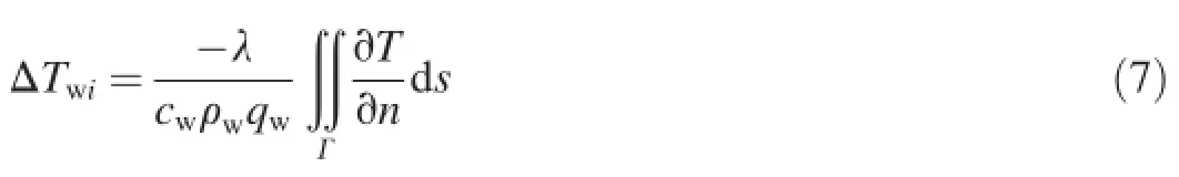
Because the pipe in the embedded model is virtual，which means that the heat exchange boundary does not actually exist in the finite element，Eq.（7）has to be modified.The heat exchange boundary of the pipe is defined as the third-type boundary condition.Therefore，

where β is the surface heat exchange coefficient of the pipe wall（kJ/（h·m2·°C），and k is the thermal conductivity of concrete（kJ/（h·m·°C））.

Eq.（8）is substituted into Eq.（7），and then the water temperature increment can be expressed as

Because the water temperature variation in one pipeembedded element is so little over one time step that it can be ignored，the water temperature increment can be approximated as

where a is the pipe radius（m），l is the length of the pipe segment in the element（m），and T′is the temperature of the pipe wall（°C）.

If a cooling pipe is divided into m segments，and the water temperature at the pipe inlet is Tw0，then the water temperature in the ith pipe segment is

The following steps are conducted in the calculation of the concrete temperature field with the embedded model，taking into account the water temperature variation along the pipe:

（1）It is assumed that the initial water temperature in all pipe segments equals the inlet water temperature of the pipe. Then，the water temperaturefor a time step is obtained with Eq.（10）and Eq.（11）.

（2）The water temperature along the pipe at the previous step is considered the boundary condition for the next iterative step.The water temperaturefor the next iterative step is calculated again.

（3）The water temperatures from the two iterations are compared.If the maximum difference satisfies a designated tolerance ε，i.e.，

the iteration at the current time step is completed.Otherwise，the above steps should be repeated.

2.2.Verification with a practical project

In order to evaluate the precision of the improved embedded model，both the explicit model with high precision and the on-site measured data from a pumping station base board were used.The base board on the field and the initial finite element model without pipes are shown in Fig.2.The finite element model included 12 504 elements and 14 632 nodes.Because of the symmetry，only half of the board was modeled.The length，width，and thickness of the base board were 36.0 m，14.0 m，and 1.5 m，respectively.There was a 0.3 m-thick concrete cushion under the base board.The dimensions of the rock base under the board were 150 m×75 m×50 m（length×width×thickness）.

Fig.2.Base board in construction and its finite element model.

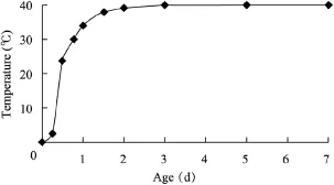
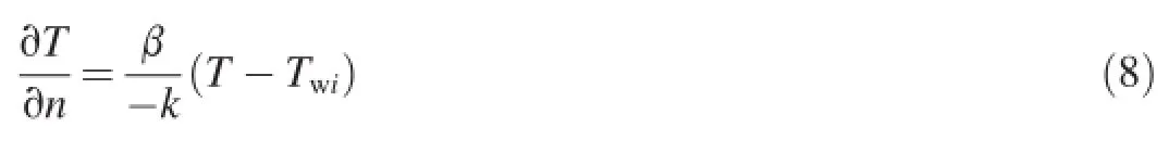
Fig.3.Adiabatic temperature rise curve of concrete.

The concrete adiabatic temperature rise curve is shown in Fig.3.The thermal conductivities of concrete and the rock base were 9.50 and 6.92 kJ/（h·m·°C），respectively.The thermal diffusivities of concrete and the rock base were 0.003 3 and 0.004 2 m2/h，respectively.The construction process in the simulation was the same as that in the practical situation. The concrete surface was covered with geotextile in the first 14 d.Then，the covering material was removed.The surface heat exchange coefficients of concrete were 28.3 and 48.91 kJ/（h·m2·°C）with and without the covering material，respectively.The initial temperature of concrete was 31.0°C. The pipe cooling treatment remained for 5 d after the casting of concrete.The measured air temperature，which was used in the numerical simulation，is shown in Fig.4.

The explicit model and improved embedded model were respectively employed to simulate four cooling pipes in the base board.After the explicit model was inserted into the initial finite element model，the numbers of elements and nodes increased to 17 016 and 19 728，respectively，while，for the improved embedded model，the numbers of elements and nodes remained unchanged.

To verify the validity and evaluate the precision of the improved embedded model，three temperature sensors，A，B，and C，were embedded at different depths on the feature section of the base board（Fig.5），but sensor C was damaged during the construction.

Fig.6 shows the simulation results of temperature variation at the locations of sensors A and B in the two models.According to measured data，the peak temperature from sensor B appears at 1.08 d，while the calculated peak temperature occurs at 1.00 d.The measured peak temperature from sensor B and the simulated values from the explicit model and the improved embedded model are 51.0°C，52.0°C，and 51.7°C，respectively.The error of the two numerical methods can satisfy the engineering requirements.

Fig.4.Air temperature for first 14 d.

Fig.5.Locations of three sensors on feature section.

Fig.6.Temperature duration curves at locations of sensors A and B.

During the test，the same inlet temperature was adopted for different cooling pipes，and there was little difference between the outlet temperatures of different pipes.Thus，we used the middle cooling pipe in the base board as an example for comparative analysis.As can be seen from Fig.7，the pipe outlet water temperatures from two numerical methods agreewith each other.The maximum difference is 1.2°C.The measured outlet water temperature varies significantly with age because of air temperature and sunlight.The calculated curves develop along the middle path of these scattered measured values，and can reflect the water temperature variation law.

Fig.7.Water temperature duration curves at pipe inlet and outlet.

Because the element number of the improved embedded model is much less than that of the explicit model，the time cost in analysis greatly decreases with the improved embedded model.Therefore，the improved model is applicable to highefficiency simulation of temperature fields in engineering projects.

3.p-version improved embedded model

The spatial temperature gradient around the pipe varies sharply during the cooling process.However，in the pipeembedded element，the temperature field is fitted with a linear function.The computation error is large if a common linear element with a large size is used.It is necessary to improve the precision of temperature field calculation based on large pipe-embedded elements in large-scale concrete structures，such as concrete dams or bridge abutments.

The principle of the p-version FEM to improve the computation precision is the addition of base functions in some elements instead of grid refinement（Zienkiewicz et al.，1983）.In recent years，this method has been introduced into structural mechanics analysis（Chen and Chen，1999，2001；Fei and Chen，2003），seepage analysis（Fei and Chen，2003；Xu and Chen，2006），rock engineering analysis（Fei et al.，2004），nonlinear vibrations（Ribeiro and Bellizzi，2010；Stojanovic et al.，2013），and composite structure analysis（Yazdani et al.，2014）.The p-version FEM has even been introduced into the boundary element method（Holm et al.，2008）.

On the basis of the p-version FEM for an unsteady temperature field simulation（Zhang and Qiang，2009），the pversion concept was introduced into the embedded model in this study.The pipe-embedded element was treated as the hierarchical element.The most common element in the simulation of the temperature field and stress field is the hexahedron element.The hierarchical format of the hexahedron element will therefore be explained in detail.

As for the concrete temperature field with the hierarchical element employed in this study，the temperature field function can be defined as

where φiis the ith base function in an element，Tiis the correspondingtemperature，andfe（p）isthenumberofbasefunctions in the element，including the point base function，line base function，face base function，and volume base function（Chen and Chen，1999；Vu and Deeks，2008；Chen et al.，2010）.

It is worth mentioning that the number of base functions may be different in different elements.However，the number of entity nodes for an element is a constant，and the coordinates of arbitrary points in the element can be obtained by interpolation with the eight entity nodes.

During the self-adaption course，the temperature field computation error，based on Chen and Chen（2001），is defined as

where T*is the analytical solution of temperature.

Based on the algorithm above，the p-version self-adaption code for the temperature field simulation using the improved embedded model is compiled with the Fortran language.

4.Numerical sample verification

4.1.Finite element model

As shown in Fig.8，four different finite element models of a concrete abutment with the dimensions of 12.0 m×9.0 m× 13.0 m（length×width×height）were created.The thickness of the rock base was 13.0 m along the Z axis.There were eight cooling pipes embedded in the concrete structure（Fig.9）. Both the horizontal and vertical distances between the cooling pipes were 1.5 m.

The explicit model of cooling pipes was applied in model 1，as shown in Fig.8（a）.In the explicit model，the grid around the pipe was refined with two circles，three circles，and five circles of elements in the pipe cooling cases.Every circle around thepipe includes four hexahedron elements.Detailed element and node numbers of different refined grids are listed in Table 1.

Fig.8.Four different finite element models.

Fig.9.Layout of cooling pipes in two different models.

The p-version improved embedded model was applied in models 2 through 4.The surface elements in these models were not refined.Compared with model 2，the element number along the X axis was reduced in model 3，and the element number along the Z axis was further reduced in model 4.In model 2，there was one pipe segment in one pipe-embedded element，while in model 3 and model 4，the numbers were two and four in one pipe-embedded element，meaning that an element with larger size contains more pipe segments，requiring a higher-order FEM for computation.

4.2.Boundary conditions and material parameters

The initial temperature of the rock base was 18°C.All surfaces of the rock base except for the top surface were insulated.The air temperature Tais set by the following equation:

where t is time（month）.

The concrete adiabatic temperature rise is

where τ is the concrete age（d）.

The thermal conductivities of the concrete abutment and rock base were 11.87 and 12.29 kJ/（h·m2·°C），respectively. The thermal diffusivities of the concrete abutment and rock base were 0.005 1 and 0.005 3 m2/h，respectively.

4.3.Case analysis

Four different cases were designed for temperature field simulation using different models in different situations.

In case 1，the thickness of each concrete layer was 3.0 m，and the time interval between the casting of two successive layers was 4 d.The initial concrete temperature was 20.0°C.In the first 2 d of casting of each layer，insulation measures were taken.No pipe cooling measures were applied in this case.

In case 2，the casting course was the same as that in case 1，and two plastic pipes，with both horizontal and vertical distances of 1.5 m，were inserted during the casting of each layer. Cooling began at 1 d after the casting of each layer and lasted for 7 d.The flow direction of pipe water was unchanged during the cooling process.The flux remained 20 m3/s.The water temperature at every pipe inlet remained 5.0°C.

In case 3 and case 4，the inlet water temperatures were 10.0°C and 20.0°C，respectively.Other conditions were the same as those in case 2.

Some feature points were used in the results analysis.The locations of these points are listed in Table 2.

4.4.Results and discussion

（1）No pipe cooling measures were applied in case 1.The grid densities near the surface of the four models were different.Temperature duration curves at feature point 1 from four models in case 1 are shown in Fig.10.It can be seen that once the cast layer with point 1 located is covered by an upper cast layer，the curves agree with one another.The difference between temperature peaks from model 2 and model 3 was about 0.3°C，and the difference between the values from model 2 and model 4 was about 0.2°C，indicating that the pversion algorithm can fit grids with different sizes well in the temperature field simulation.

（2）In case 2，different grid refinement schemes of model 1 were applied around the cooling pipe.Fig.11 shows the temperature difference duration curve at feature point 5 near the center of the concrete abutment.The figure indicates that the computed temperature difference between two grid refinement schemes is less than 0.1°C，when the numbers of circles in the two grid refinement schemes are not less than three.Considering that the time cost in the five-circle grid refinement scheme is much greater than that in the three-circle grid refinement scheme，the latter is relatively efficient，andcan be used for comparison with the p-version improved embedded model.

Table 1Information on test models.

Table 2Coordinates of feature points.

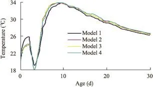
Fig.10.Temperature duration curves at feature point 1 from different models in case 1.

Fig.11.Temperature difference duration curves at feature point 5 from different grid refinement schemes of model 1 in case 2.

（3）The peak temperatures at feature points 1 and 4 from four models in four cases are listed in Table 3.It can be seen that the temperature difference near the upstream concrete surface in different cases is less than 1.0°C，and the value near the center of the horizontal cross-section of the concrete abutment is less than 0.5°C.From the comparison of peak temperatures and temperature duration curves，it can be concluded that the method proposed in this paper can obtain satisfying precision for a mass concrete structure containing cooling pipes.

（4）Fig.12 shows the temperature contours of the y=4.5 m section 13.5 d after the casting of the last concrete layer in case 2.The dots in Fig.12（a）show the cross-section of cooling pipes.It can be seen that the contour shape and numerical values from the four models are similar.It should be pointedout that the contour post-processing of the four models still relies on the simulation results of the entity point，because no suitable post-processing tool has been developed for the pversion FEM.

Table 3Peak temperatures at feature points.

（5）The total time costs of different models in cases 2 through 4 are listed in Table 4，showing that the p-version improved embedded model saves a significant amount of time throughout the analysis.For example，the time cost of model 1 in case 2，using the three-circle grid refinement scheme，is 750.16 s，while the time cost of model 4 is 335.15 s，meaning that the total analysis efficiency using the p-version embedded model is doubled，while precision remains the same.At the same time，the preprocessing course of the finite element model can be simplified.The test sample in this paper is arelatively small structure.When the proposed method is applied to a larger engineering structure，such as a large concrete dam，the efficiency improvement in model construction and analysis will be much more remarkable.

Fig.12.Temperature fields of y=4.5 m section 13.5 d after casting of last concrete layer in case 2 from different models（units:°C）.

Table 4Computation time cost by different models in different cases.

5.Conclusions

The p-version self-adaption idea was introduced into the improved embedded model for the simulation of concrete temperature fields containing cooling pipes.The corresponding algorithm was deduced，and the initial values and boundary conditions were investigated.Based on the algorithm，the program was compiled with the Fortran language. The comparison of some numerical samples shows that the proposed model can provide satisfying precision and a higher efficiency.

The proposed approach creates greater convenience in the preprocessing of the finite element model from two aspects. First，more than one pipe segment can be arranged in one embedded model element，which is a pronounced improvement.When different pipe layout schemes in a concrete structure need to be simulated，it is unnecessary to create different grids in the structure to accommodate every kind of pipe layout.Second，the element that contains pipe segments does not need so regular a shape as in the explicit model，decreasing the difficulty in modeling and grid creation，especially for complicated structures.

References

Abbas，B.M.，Al-Mahaidi，R.S.，2007.Internal temperature rise and early thermal stresses in concrete.In:Proceedings of the 4th International Structural Engineering and Construction Conference，ISEC-4:Innovations in Structural Engineering and Construction.Taylor and Francis/Balkema，Melbourne，pp.395-400.

Bentz，D.P.，Weiss，W.J.，2008.REACT:Reducing early age cracking today. Concr.Plant Int.（3），56-61.

Bureau of Reclamation，1988.Concrete Manual.U.S.Department of the Interior，Washington，D.C.

Chen，G.R.，2009.Principle and Application of Finite Element Method.Science Press，Beijing（in Chinese）.

Chen，S.H.，Chen，Z.，2001.Study on p-version adaptive finite element method for analysis of hydraulic structure.J.Hydraul.Eng.32（11），62-70（in Chinese）.

Chen，S.H.，Qin，N.，Xu，G.S.，Shahrour，I.，2010.Hierarchical algorithm of composite element containing drainage holes.Int.J.Numer.Methods Biomed.Eng.26（12），1856-1867.http://dx.doi.org/10.1002/cnm.1271.

Chen，S.H.，Su，P.F.，Shahrour，I.，2011.Composite element algorithm for the thermal analysis of mass concrete simulation of cooling pipes.Int.J. Numer.Methods Heat Fluid Flow 21（4），434-447.http://dx.doi.org/ 10.1108/09615531111123100.

Chen，Z.，Chen，S.H.，1999.3-D hierarchical FEM analysis for hydraulic structure.J.Hydraul.Eng.30（12），53-58.http://dx.doi.org/10.3321/ j.issn:0559-9350.1999.12.010（in Chinese）.

Fei，W.P.，Chen，S.H.，2003.3-D p-version elasto-viscoplastic adaptive FEM model for hydraulic structures.J.Hydraul.Eng.34（3），86-92.http:// dx.doi.org/10.3321/j.issn:0559-9350.2003.03.016（in Chinese）.

Fei，W.P.，Zhang，L.，Xie，H.P.，2004.A p-version adaptive finite element method and its application to rock and soil engineering.Rock Soil Mech.25（11），1727-1732.http://dx.doi.org/10.3969/j.issn.1000-128X. 2007.02.002（in Chinese）.

Holm，H.，Maischak，M.，Stephan，E.P.，2008.Exponential convergence of the h-p version BEM for mixed boundary value problems on polyhedrons. Math.Methods Appl.Sci.31（17），2069-2093.http://dx.doi.org/10.1002/ mma.1009.

Hossain，A.B.，Weiss，J.，2004.Assessingresidualstress developmentandstress relaxation in restrained concrete ring specimens.Cem.Concr.Compos. 26（5），531-540.http://dx.doi.org/10.1016/S0958-9465（03）00069-6.

Kim，J.K.，Kim，K.H.，Yang，J.K.，2001.Thermal analysis of hydration heat in concrete structures with pipe-cooling system.Comput.Struct.79（2），163-171.http://dx.doi.org/10.1016/S0045-7949（00）00128-0.

Lin，P.，Li，Q.B.，Jia，P.Y.，2014.A real-time temperature data transmission approach for intelligent cooling control of mass concrete.Math.Probl. Eng.2014，514606.http://dx.doi.org/10.1155/2014/514606.

Liu，N.，Liu，G.T.，1997.Sub-structural FEM for the thermal effect of cooling pipes in mass concrete structures.J.Hydraul.Eng.28（12），43-49（in Chinese）.

Mai，J.X.，1998.A combined method of theoretic and numerical solutions for pipe cooling in concrete dams.J.Hydroelectr.Eng.（4），31-41（in Chinese）.

Myers，T.G.，Fowkes，N.D.，Ballim，Y.，2009.Modeling the cooling of concrete by piped water.J.Eng.Mech.135（12），1375-1383.http://dx.doi.org/ 10.1061/（ASCE）EM.1943-7889.0000046.

Ribeiro，P.，Bellizzi，S.C.B.，2010.Non-linear vibrations of deep cylindrical shells by the p-version finite element method.Shock Vib.17（1），21-37. http://dx.doi.org/10.3233/SAV-2010-0495.

Stojanovic，V.，Ribeiro，P.，Stoykov，S.，2013.Non-linear vibration of Timoshenko damaged beamsbyanew p-version finiteelement method.Comput.Struct.120，107-119.http://dx.doi.org/10.1016/ j.compstruc.2013.02.012.

Townsend，C.L.，1981.Control of Cracking in Mass Concrete Structures. United States Department of the Interior，Bureau of Reclamation，Denver.

Vu，T.H.，Deeks，A.J.，2008.A p-hierarchical adaptive procedure for the scaled boundary finite element method.Int.J.Numer.Methods Eng.73（1），47-70.http://dx.doi.org/10.1002/nme.2055.

Weiss，W.J.，Bentz，D.，Schindler，A.，Lura，P.，2012.Internal curing:Constructing more robust concrete.Struct.Mag.（1），10-14.

Xu，G.S.，Chen，S.H.，2006.Seepage analysis considering drainage holes by pversion adaptive composite element method.Chin.J.Rock Mech.Eng. 25（5），969-973（in Chinese）.

Yang，J.，Hu，Y.，Zuo，Z.，Jin，F.，Li，Q.B.，2012.Thermal analysis of mass concrete embedded with double-layer staggered heterogeneous cooling water pipes.Appl.Therm.Eng.35，145-156.http://dx.doi.org/10.1016/ j.applthermaleng.2011.10.016.

Yazdani，S.，Ribeiro，P.，Rodrigues，J.D.，2014.A p-version layerwise model for large deflection of composite plates with curvilinear fibres.Compos.Struct. 108（1），181-190.http://dx.doi.org/10.1016/j.compstruct.2013.09.014.

Zhang，Y.，Qiang，S.，2009.Research on 3D p-version hierarchical FEM for unsteady temperature field.Rock Soil Mech.30（2），487-491.http:// dx.doi.org/10.3969/j.issn.1000-7598.2009.02.035（in Chinese）.

Zhu，B.F.，1999.Thermal Stresses and Temperature Control of Mass Concrete. China Electric Power Press，Beijing（in Chinese）.

Zhu，Y.M.，Liu，Y.Z.，Xiao，Z.Q.，2004.Analysis of water cooling pipe system in mass concrete.In:Wieland，M.，Ren，Q.W.，Tan，J.S.Y.，Eds.，Proceedingsofthe4th InternationalConference on Dam Engineering:New Development in Dam Engineering.CRC Press，pp.1205-1210.

Zhu，Z.Y.，Qiang，S.，Chen，W.M.，2013.A new method solving the temperature field of concrete around cooling pipes.Comput.Concr.11（5），441-462.http://dx.doi.org/10.12989/cac.2013.11.5.441.

Zienkiewicz，O.C.，Gago，J.P.，de，S.R.，Kelly，D.W.，1983.The hierarchical concept in finite element analysis.Comput.Struct.16（1-4），53-65.http:// dx.doi.org/10.1016/0045-7949（83）90147-5.

This work was supported by the National Natural Science Foundation of China（Grant No.51109071）.

*Corresponding author.

E-mail address:sqiang2118@163.com（Sheng Qiang）.

Peer review under responsibility of Hohai University.

http://dx.doi.org/10.1016/j.wse.2015.08.001

1674-2370/©2015 Hohai University.Production and hosting by Elsevier B.V.This is an open access article under the CC BY-NC-ND license（http:// creativecommons.org/licenses/by-nc-nd/4.0/）.