Uniqueness，scale，and resolution issues in groundwater model parameter identification

Tian-hyi J.Yeh*，De-qiang Mao，Yuan-yuan Zha，Jet-hau Wen，Li Wan，Kuo-hin Hsu，Cheng-haw Lee

aDepartment of Hydrology and Water Resources，The University of Arizona，Tucson 85721，USA

bDepartment of Resources Engineering，National Cheng Kung University，Tainan 701，PR China

cDepartment of Geophysics，Colorado School of Mines，Golden 80401，USA

dState Key Laboratory of Water Resources and Hydropower Engineering Science，Wuhan University，Wuhan 430072，PR China

eDepartment of Safety Health and Environmental Engineering，National Yunlin University of Science and Technology，Touliu 64002，PR China

fResearch Center for Soil&Water Resources and Natural Disaster Prevention，National Yunlin University of Science and Technology，Touliu 64002，PR China

Received 19 June 2015；accepted 17 July 2015

Available online 14 August 2015

Uniqueness，scale，and resolution issues in groundwater model parameter identification

Tian-chyi J.Yeha，b，*，De-qiang Maoc，Yuan-yuan Zhaa，d，Jet-chau Wene，f，Li Wanc，Kuo-chin Hsub，Cheng-haw Leeb

aDepartment of Hydrology and Water Resources，The University of Arizona，Tucson 85721，USA

bDepartment of Resources Engineering，National Cheng Kung University，Tainan 701，PR China

cDepartment of Geophysics，Colorado School of Mines，Golden 80401，USA

dState Key Laboratory of Water Resources and Hydropower Engineering Science，Wuhan University，Wuhan 430072，PR China

eDepartment of Safety Health and Environmental Engineering，National Yunlin University of Science and Technology，Touliu 64002，PR China

fResearch Center for Soil&Water Resources and Natural Disaster Prevention，National Yunlin University of Science and Technology，Touliu 64002，PR China

Received 19 June 2015；accepted 17 July 2015

Available online 14 August 2015

Abstract

This paper first visits uniqueness，scale，and resolution issues in groundwater flow forward modeling problems.It then makes the point that non-unique solutions to groundwater flow inverse problems arise from a lack of information necessary to make the problems well defined. Subsequently，it presents the necessary conditions for a well-defined inverse problem.They are full specifications of（1）flux boundaries and sources/sinks，and（2）heads everywhere in the domain at at least three times（one of which is t=0），with head change everywhere at those times being nonzero for transient flow.Numerical experiments are presented to corroborate the fact that，once the necessary conditions are met，the inverse problem has a unique solution.We also demonstrate that measurement noise，instability，and sensitivity are issues related to solution techniques rather than the inverse problems themselves.In addition，we show that a mathematically well-defined inverse problem，based on an equivalent homogeneous or a layered conceptual model，may yield physically incorrect and scenario-dependent parameter values.These issues are attributed to inconsistency between the scale of the head observed and that implied by these models.Such issues can be reduced only if a sufficiently large number of observation wells are used in the equivalent homogeneous domain or each layer.With a large number of wells，we then show that increase in parameterization can lead to a higher-resolution depiction of heterogeneity if an appropriate inverse methodology is used.Furthermore，we illustrate that，using the same number of wells，a highly parameterized model in conjunction with hydraulic tomography can yield better characterization of the aquifer and minimize the scale and scenario-dependent problems.Lastly，benefits of the highly parameterized model and hydraulic tomography are tested according to their ability to improve predictions of aquifer responses induced by independent stresses not used in the inverse modeling efforts.

©2015 Hohai University.Production and hosting by Elsevier B.V.This is an open access article under the CC BY-NC-ND license（http:// creativecommons.org/licenses/by-nc-nd/4.0/）.

Uniqueness；Scale；Resolution；Forward and inverse problems；Hydraulic tomography

1.Introduction

The need of using inverse models to determine the spatial distribution of hydraulic properties has been well recognized for decades.Nevertheless，as stated by Carrera and Neuman（1986），“There is a general consensus among groundwater modelers that the inverse problem may，at times，result in meaningless solutions.However，the reasons for this“misbehavior”of the inverse solution are not always well understood:some hydrologists attribute them to nonuniqueness，some to nonidentifiability，and others to instability.This misunderstanding has led to a controversy in the literature regarding the question whether the inverse problem is at all solvable；if so，under what circumstances and in what manner. There are those who argue that this problem is hopelessly illposed and，as such，intrinsically unsolvable.”After more than two decades，arguments remain.This controversy mainly stems from the definition of a well-posed mathematic problem given by Hadamard（1902）:mathematical models of physical phenomena should have the properties that（1）a solution exists，（2）the solution is unique，and（3）the solution depends continuously on the data，in some reasonable topology.The last condition implies that if the solution depends in a discontinuous way on the data，then small errors，whether rounding-off errors，measurement errors，or perturbations caused by noise，can create large deviations.Most of the inverse models in science exhibit this unstable nature.The inverse problem in subsurface hydrology is therefore commonly perceived as an ill-posed problem.

In spite of the ill-posed nature of inverse problems，Nelson（1960）demonstrated mathematically five decades ago that three-dimensional（3D）heterogeneous hydraulic conductivity distribution can be uniquely identified if the spatial potential variation is known，and the hydraulic conductivity at one point in every stream tube under a steady flow is given.While recognizing that an insufficient amount of Cauchy data causes the inverse problem of steady flow to be non-unique，Neuman（1973）attributed an infinite number of possible solutions of the inverse problem to errors in data and governing equations. Because the inverse modeling efforts are non-unique，Emsellem and de Marsily（1971）and Neuman（1973）emphasized the need for multiple objectives in dealing with groundwater parameter identification problems:calibration error and physical plausibility of the estimate.

An extensive discussion on the uniqueness，identifiability，and stability associated with inverse modeling of transient and steady groundwater flow equations was provided by Carrera and Neuman（1986）.They stated that identifiability is ensured if the rank of the Jacobian matrix is equal to the number of unknown parameters.They concluded，however，that“The large number of flow situations that can arise from governing groundwater flow equations prevents us from developing detailed rules about uniqueness.”They further stated that“No parameter estimates must be accepted at face value without subjecting them first to a thorough sensitivity analysis…Concerning the sensitivity of heads to model parameters，the issue is strongly problem-dependent and can be resolved only through a prior and/or post-optimal sensitivity analysis.”

Likewise，McLaughlin and Townley（1996）and Carrera et al.（2005）stressed that the low sensitivity of head to the hydraulic conductivity is the cause of the difficulties in solving groundwater inverse problems.In particular，McLaughlin and Townley（1996）stated“In many situations where parameters are difficult to identify it is easier to improve sensitivity by introducing new kinds of information than by simply adding more measurements of the same variable.This is particularly true in the groundwater flow inverse problem.Since steady state heads are relatively insensitive to spatial variations in hydraulic conductivity，estimation performance may not improve dramatically when more head measurements are included.”They also suggested inverse experiments should be designed so as to maximize the sensitivity of measurements to estimated parameters（Knopman and Voss，1988）.More recently，the role of different statistics based upon sensitivity in parameter identifiability have been discussed by Doherty and Hunt（2009），Hill（2010），and Doherty and Hunt（2010）.

Stallman（1956）noted that his inverse solutions tended to be unstable.He suggested that this instability problem can be prevented by treating transmissivity as a constant over large segments of the aquifer（zones）and using least squares to estimate transmissivity over such zones.The zone must not be too large.Otherwise，important information about spatial variability is lost and one may be unable to obtain a satisfactory match between computed and measured heads（a sparsely parameterized approach）.This is basically a block parameterization or zonation approach（Neuman，1973；Hill，2006；Sun and Yeh，1985；Eppstein and Dougherty，1996；McLaughlin and Townley，1996）.In particular，McLaughlin and Townley（1996）stated“If the actual spatial distribution of hydraulic conductivity is not blocked or if the block boundaries are incorrectly specified，the inverse algorithm may be forced to generate unrealistic estimates in order to provide a good fit to head measurements.So，although the inverse problem may be well-posed in the sense that it yields a stable solution，the estimates it provides may not properly characterize the subsurface environment.”They further suggested that“when geological structure is apparent and formation boundaries are distinct a blocked approach to parameterization is probably the best choice.”

On the other hand，highly parameterized approaches such as geostatistical approaches（e.g.，kriging，cokriging，conditional simulations，and geostatistics-based inverse models）have been used extensively over the past few decades（Zimmerman et al.，1998）.Hunt et al.（2007）recently emphasized the need for increasing parameterization in groundwater model calibrations with the use of a regularized inverse approach.

The objective of this paper is not to provide a review of mathematical methods for solving groundwater inverse problems as there are already many review articles.Rather，it is to emphasize the fact that non-unique solutions in either a forward or an inverse problem are a result of the lack of data that satisfy necessary conditions for a well-defined problem. Mathematical stability issues or high or low measurement sensitivity to the estimated parameters are not the cause.The non-uniqueness of forward and inverse problems should be addressed as uncertainty in the solutions.

In this paper，we first visit the forward groundwater flow model，the necessary conditions for a forward solution to be well defined，and the process scale implied in the conceptual model.We then emphasize the fact that forward modeling ofany field problems is often mathematically ill-conceived in the Hadamard sense，since the problems often do not have sufficient information.In addition，they inherently suffer from scale differences between simulated and observed heads，and from differences in spatial resolution between simulated and true head distributions due to our conceptualization of the real flow process.

Afterward，we present the necessary conditions for a groundwater flow inverse problem that should be well defined and numerical examples that corroborate these conditions.We also show that a mathematically well-defined inverse problem，based on an equivalent homogeneous or a sparsely parameterized conceptual model（e.g.，a layered geologic model），may yield a physically incorrect solution due to inconsistency between the scale of the process observed and that implied by a conceptual model.

In order to avoid the scale issues，we demonstrate that sufficient spatial data（i.e.，observation wells）are necessary. With the same number of spatial data，we show that a highly parameterized inverse model can produce more detailed aquifer heterogeneity than a sparely parameterized model. More importantly，if data collections（e.g.，aquifer tests）are conducted in a tomographic fashion，the responses from the same monitoring network carry non-redundant information about the aquifer heterogeneity.With this non-redundant information，a highly parameterized model yields a higherresolution description of aquifer heterogeneity than the one without the non-redundant dataset.The theme of this paper is therefore to promote intelligent approaches to collect and analyze data in order to enhance characterization of aquifer heterogeneity.

2.Uniqueness，scale，and resolution issues of forward problems

2.1.Governing flow equations for forward problems and control volume（CV）

A forward problem here refers to solving governing flow equations for the head in time and space over a solution domain（i.e.，a basin，or an arbitrarily defined field site），with given parameters，boundaries，and initial conditions.The partial differential equation used to describe the movement of water in multi-dimensional，fully saturated，geologic porous media is

with boundary conditions

and initial condition where x is the position vector，t is time，K（x）is the hydraulic conductivity，H（x，t）is the total head，Q（x，t）is a sink or source，Ss（x）is the specific storage，H*（x，t）is the prescribed head at boundary Γ1，q（x，t）is the boundary flux at boundary Γ2，and n is a unit vector normal to Γ2.K（x）and Ss（x）are defined as properties or parameters，and H（x，t）are state variables or system responses.

While mathematically，H（x，t），K（x），and Ss（x）are defined at a point x，they conceptually and physically represent averages over a small volume of geologic medium，centered at x in a domain（e.g.，a sandbox）.This volume for K（x）and Ss（x），denoted as a CVat point x，ought to be larger than many pores but much smaller than the entire sandbox.Within this CV，the hydraulic parameters（K and Ss）are considered as constants（i.e.，homogeneous）.We in essence use this CV to blur irregular and discrete pores and channels such that the medium in the sandbox can be viewed as being continuous in space（i.e.，Darcian continuum）.

We then carry out the mass balance analysis over this CV and apply Darcy's law to yield a head distribution inside this CV for a given flux.Notice that the head is also a volumetric attribute as implied in fluid continuum concept.It represents an averaged energy of many water molecules within a volume. This volume over which the head is defined must be smaller than the CV but much larger than many water molecules. Additionally，the head of this volume at a given location x and time t，H（x，t），within the CV also represents an ensembleaveraged head at x and t in this CV of the sandbox.For example，consider a CV that contains 100 pebbles of different shapes.These pebbles can be distributed differently and yield different pore distributions.As we apply Darcy's law to this CV，we essentially assume a uniform K and a smooth head profile，regardless of how the pores are distributed in the CV. Different pore distributions yield different irregular head profiles.This head profile based on Darcy's law is an average of all different head profiles，resulting from all possible pore distributions.As such，a head based on Darcy's law at a location and time in the CV is an average of all possible heads（ensemble average head）at that location and time，corresponding to different pore distributions within the CV.

2.2.Representative elementary volume（REV）and conceptual models

If the parameter value defined by a CV varies with the location in the sandbox，the medium of the sandbox is said to be heterogeneous at this given size of CV.K（x）or Ss（x）of this heterogeneous medium is thus a spatial variable，which may have a spatially constant mean（i.e.，spatially stationary）or a spatially variable mean（i.e.，spatially nonstationary）.In the stationary case，one may increase the size of the CV（i.e.，scale）to redefine a new value for the parameter.If the value defined by this new CV does not vary with locations in the sandbox，excluding locations near boundaries，the previously defined heterogeneous medium then becomes a homogeneous medium with this new CV.This CV is called the REV of the medium（Bear，1972；de Marsily，1986）.Here，we will call itthe spatial REV.That is，the property defined over the REV is a spatially translational invariant.The term elementary implies that the size of the REV is much smaller than the entire medium.In other words，REVis a CV that is sufficiently large but smaller than the domain such that characteristics（e.g.，spatial statistics）within the volume are representative of the entire population（the domain）.In cases where heterogeneity is nonstationary，spatial REVs may exist within locally stationary parts of the medium（e.g.，zones，layers，formations，etc.）but not for the entire medium.That is，no spatial REV exists for the entire domain.Note that here we ignore anisotropy at this CV scale since we assume that its effects are small compared with the effects of spatial variability of the parameter value under this CV in the domain.

Regardless of the fact that a field is nonstationary，the homogeneity assumption has been widely invoked for the sake of mathematical convenience and practicality（e.g.，in applications of the Theis solution to field pumping tests）.In these applications，the entire medium is conceptualized as homogeneous based on a CV as large as the field site（i.e.，the domain）.Since the characteristics within this CVare the same as the entire domain，we can call this CVa domain-sized REV. In this case，the requirement for an REVof being elementary is met only in the ensemble sense，rather than in the spatial sense，as in the stationary case.That is，the heterogeneity within the domain is merely a realization of many possible heterogeneous fields.These possible fields have the same statistical distribution，e.g.，mean，variance，and correlation scales，but have different spatial distributions.Thus，the domain-sized REV is also called an ensemble REV.The parameter associated with this ensemble REV represents an average of all possible parameter distributions over the domain.This parameter is generally referred to as the effective parameter for an equivalent homogeneous medium.Since the entire domain is assumed to be homogenous，domain-scale anisotropy in the effective K is often introduced to accommodate effects of structured heterogeneity（i.e.，layering and formations）within this REV.Furthermore，as mentioned in section 2.1，the head H（x，t）at any location x and time t in the domain represents an average of all possible heads at that location and time（ensemble average head），corresponding to all possible hydraulic property distributions within this domain-size REV.

Accordingly，an aquifer can be conceptualized as an equivalent homogeneous or a heterogeneous aquifer for forward models.The heterogeneous conceptual model can be further subdivided into a sparsely parameterized model（e.g.，by dividing a geologic medium into layers or zones）and a highly parameterized model（prescribing heterogeneity in detailbeyond the layers orzones）in the following discussions.

2.3.Uniqueness，scale，and resolution

A forward problem is well defined if the parameters and initial and boundary conditions are fully specified for the solution domain such that a particular（unique）solution exists. That is，the objective of the problem is fully specified，and theoretically it has a unique solution.Otherwise，the problem is ill defined（without a clear objective）；this problem cannot be solved unless these conditions are assumed.Since many possible conditions can be assumed，the problem then has an infinite number of possible solutions（non-unique solutions）. Such an ill-defined forward problem is thus an ill-posed problem according to Hadamard's definition，regardless of whether the solution is stable or not.

On the other hand，because of the stability issue of the solution，a well-defined forward problem may not guarantee a solution，nor does it warrant a correct solution，although the correct solution theoretically exists.For instance，a highly nonlinear relationship between the pressure head and hydraulic properties of unsaturated media often makes a welldefined forward unsaturated flow problem difficult to solve numerically:there are unstable solutions，diverging solutions，and wrong solutions.Therefore，a well-defined unsaturated flow forward problem may be ill posed in Hadamard's view. Nevertheless，such stability issues are related to solution techniques.

In applying a forward heterogeneous or homogeneous model to a real-world problem，one often finds that information on temporal and spatial variations in parameters and initial and boundary conditions are incomplete or unknown. Therefore，real-world forward problems in groundwater hydrology are often ill defined，and have non-unique solutions due to lack of information.In other words，the solution is uncertain.

In addition，forward problems suffer from scale and resolution issues.The scale issue is the difference between the predicted head at a point in space based on a conceptual model and the corresponding observed head at the point in the realworld aquifer.Specifically，an observed head generally represents an average head over many pores or heterogeneity at a point，depending on the size of the instrument（e.g.，the length of the screen interval of an observation well）and the diffusive length of the head process（Yeh et al.，2005）.On the other hand，a predicted head based on the model represents an ensemble average at a point within the CV or REV，as discussed previously.Although not proven，one may speculate that if the scale of the head measurement is sufficiently large in terms of the size of the CV or REV，the two heads may be equivalent.Otherwise，one can only expect that the spatial trend of the predicted heads approaches that of observed heads（Wu et al.，2005；Yeh et al.，2005）.

The resolution of a model is the degree of spatial details of the predicted head or flow process.This issue generally rests upon the resolution of heterogeneity specified in the forward model（i.e.，whether it is an equivalent homogeneous，sparsely parameterized，or highly parameterized conceptual model）.In principle，the finer specified heterogeneity（the smaller CV）is，the higher the resolution of the predicted head is，even though the scale issue may remain but becomes less significant.

Uniqueness，scale，and resolution issues for the forward problems are not new.Over the past few decades，variousstochastic approaches have been developed to tackle these issues associated with forward problems.For example，Yeh et al.（1985a，1985b，1985c），Gelhar（1993），Wu et al.（2005），Yeh et al.（2005）and many others have developed methods for estimating the unconditional effective parameters and uncertainty in prediction due to the unknown spatial distribution of the parameter.Similarly，various stochastic conditional approaches，using hydrologic observations，have been developed to derive the most probable solution and uncertainty for this ill-defined problem.For instance，for aquifers，see Delhomme（1979），Smith and Schwartz（1981a，1981b），Dagan（1982），Wagner and Gorelick（1989），Graham and McLauglin（1989），Jang and Liu（2004）；for the vadose zone，see Harter and Yeh（1996），Li and Yeh（1999）.The unconditional effective parameter approaches aim to drive statistically unique predictions at a low spatial resolution while the conditional approaches target predictions at a higher spatial resolution.

3.Uniqueness of solution to inverse problems

Here，an inverse problem is referred to as solving Eq.（1）for K（x）or K（x）and Ss（x），using H information and initial and boundary conditions.This section demonstrates that as long as this inverse problem is well defined，a unique and mathematically correct solution can be obtained.Specifically，we first identify necessary conditions for a well-defined inverse problem of an equivalent homogeneous conceptual model.Then，we illustrate the existence of the unique solution for this problem in spite of high or low sensitivity and noise in data.Discussions of conditions for uniqueness of the inverse solution of a heterogeneous conceptual model then follow.We visit the scale and resolution issues of the inverse problem in section 4.

3.1.Equivalent homogeneous conceptual models

The inverse model based on the equivalent homogeneous conceptual model can be formulated as a system of linear equations or nonlinear equations.

3.1.1.System of linear equations

Based on the forward model（Eq.（1）），the inverse equation for the homogeneous media is

3.1.2.System of nonlinear equations

An alternative to the system of linear equations approach is to solve the following nonlinear equation（s）for K and Ssvalues:

where H（xi，tj）is the observed head at xiand tj；H（xn，tm）is the observed head at xnand tm；and i，j，n，and m are subscripts， denoting different locations and times.is the calculated head from a forward model with some estimatedvalues.The necessary conditions for these equations to be well defined are essentially identical to those established based on the system of linear equations.To demonstrate this fact，Eq.（5）was solved using a direct solution approach and a least squares approach，the latter of which permits us to examine the effect of measurement noises.

3.1.2.1.Direct solution approach

For better illustration purposes，a well-known brute-force solution mapping approach was employed to find the solution to Eq.（5）.The mapping was conducted using an analytical model for one-dimensional（1D）flow problems and a numerical forward model for two-dimensional（2D）problems.

（1）Analytical solutions:Two cases associated with flow through a 1D，semi-infinite，saturated homogeneous medium were examined.Case 1 involves the following boundary and initial conditions:

The forward solution corresponding to these conditions is

where D=K/Ssand erfc is the complementary error function.

Case 2 represents the situation where the boundary and initial conditions are

The corresponding analytical solution for the head distribution in this case is

In order to determine K and Ssusing either Eq.（7）or Eq.（9），two different heads（either from two different times at one location or from two different locations at a given time）are needed to form two independent equations.To verify this requirement，Eq.（7）or Eq.（9）was solved for observed heads，H（z，t），at some selected location and time，assuming K=0.495cm/min，Ss=0.000 1cm-1，andinitial andboundary conditions:H0=200 cm and q=-0.1 cm/min.Subsequently，we systemically varied K and Ssvalues in Eq.（7）and Eq.（9）with known initial and boundary conditions to obtain many head values at the observed location and time.If a pair of K and Ssvalues yielded the same value as the observed head，this pair of K and Ssvalues was considered to be the solution of inverse problem of Case 1 or Case 2.

For Case 1，pairs of K and Ssvalues for observed heads at five different pairs of x and t，20 cm and 0.03 min，20 cm and 0.05 min，20 cm and 10.0 min，50 cm and 10.0 min，and 55 cm and 10.0 min are depicted in Fig.1.As indicated by the curved line in the figure，an infinite number of K andSspairs exist that can reproduce an observed head at a given location and time. Nevertheless，lines created by K and Sspairs for observed heads at different times and locations intersect at the true solution:K=0.495 cm/min and Ss=0.000 1 cm-1，indicating a unique solution.

If noise or error was present in the observed head，two lines created by pairs of K and Ssvalues for two observed heads at different times or locations intersected at K and Ssvalues other than the true solution（Fig.2）.This yielded inconsistent solutions or no common solution existed.However，there was no instability issue.

For Case 2，K and Sspairs that reproduced the observed head formed a straight line on a K vs.Ssplot.All points on the line had the same K to Ssratio（i.e.，the same diffusivity）. This result held for observed heads at different locations and times.Moreover，all lines overlapped one another（this figure is omitted in this paper for space considerations）.Such overlapped lines indicate an infinite number of solutions under this scenario，which involved only prescribed head boundaries.

Fig.1.Five lines of K and Sspairs that produce heads at five different pairs of x and t intersect at true K and Ssvalues，indicating a unique solution and no instability issues.

Fig.2.Five lines of K and Sspairs that produce heads at five different pairs of x and t without single common intersection indicating no common solution.

Results of these two cases suggest that a flux boundary condition，and at least two head values at either different times at one location or two different locations at one time，are necessary to obtain a unique solution for a pair of K and Ss. Accordingly，we can deduce that the inverse solution to the Theis equation for transmissivity and storage coefficient of a homogeneous and isotropic aquifer can be unique.

（2）Numerical solutions:We next explored the prerequisites for identifying anisotropic conductivities of homogeneous media under steady and transient 2D saturated flow situations.In this case，we used a finite element program for variably saturated flow and transport in 2D（VSAFT2）（Yeh et al.，1993）as a forward model.

Fig.3 shows the simulated total head and streamlines in a non-uniform transient flow at a given late time（steady-state）in a cross-sectional aquifer with anisotropic hydraulic conductivity Kx=0.3 m/min，Kz=0.03 m/min，and Ss=0.005 5 m-1. Principaldirectionsofthehydraulicconductivitywereassumed to run in the same direction as the x and z coordinates.A total head of 100 m was assigned as the initial condition everywhere. Attimesgreaterthanzero，aconstantflux（q=0.05m/min）was imposed on the top boundary from x=0 to x=5 m，the righthand side of the domain was a constant total head boundary（100 m），and the remaining boundaries were no-flux boundary conditions.Solid circles in Fig.3 denote six nodes where head values were sampled.Sensitivities of heads at these sampling locations to change in Kx，Kz，and Ss，as a function of time，are illustrated in Figs.4（a），（b），and（c），respectively.

Using the solution mapping approach，values of possible pairs of Kxand Kzthat can reproduce six steady heads at the six sampling locations are plotted in Fig.5.Lines resulting from heads at different sampling locations intersected each other at the true Kxand Kzvalues，suggesting the existence of unique solution.Note that the head at node 123 or 125 near the constant head boundary was only slightly sensitive to change in K（close to zero；see Figs.4（a）and（b））.Using one of these heads and one head at other locations，one could still find theunique and correct solution.This seems to contradict the emphasis by previous investigators on the importance of high sensitivity，as discussed in the introduction.Nonetheless，finding the solution was difficult（but feasible）if only heads at nodes 123 and 125 were used，since lines formed by the heads at the two nodes were almost parallel（Fig.5）.

Fig.3.Total head contours and streamlines of a non-uniform，steady state flow through an equivalent homogeneous，anisotropic aquifer.（Dots indicate sampling locations.）

Fig.4.Sensitivity of head at six sampling locations（Fig.3）to change in Kx，Kz，and Ssas a function of time.（Values close to zero indicate low sensitivities.）

In the case where the flow was transient，heads at the six sampling locations and two times were used to map the solution.Sets of Kx，Kz，and Ssvalues that can yield a given head at a given set of x，z，t formed a surface.All twelve surfaces intersected at a point at the true values（Kx=0.3 m/min，Kz=0.03 m/min，and Ss=0.005 5 m-1），indicative of existence of a unique solution.At least three surfaces are necessary to intersect at the point.Therefore，three head values at different locations and times（e.g.，at（x1，z1，t1），（x2，z2，t1），and（x2，z2，t2））are needed to ensure a unique solution.

Interestingly，Fig.6 shows that surfaces generated from sets of Kx，Kz，and Ssvalues that reproduced given head values at three different times（3，6，and 10 min）at one location（node 125）still intersected at the true Kx，Kz，and Ssvalues，indicating a unique solution.An analysis of temporal evolution of∂H（x，z，t）/∂Kx，∂H（x，z，t）/∂Kz，and∂H（x，z，t）/∂Ss（Fig.4）and a close examination of the flow field（Fig.3）revealed that the flow field at the sampling location changed with time and the sensitivities changed accordingly.The change in the flow field apparently provided non-redundant information about the anisotropy even though the sensitivity of the head to parameters and its change at the sampling location had small values.

Fig.5.Lines of Kxand Kzpairs yielding six steady heads at six locations in aquifer（Fig.3）intersecting each other at true values of Kxand Kz.（There exists a unique solution without instability issues.）

Fig.6.Surfaces of sets of Kx，Kz，and Ssvalues yielding given head values at three times at one location in aquifer.（Three surfaces，the true Kx，Kz，and Ssvalues of the aquifer，intersect at one point.）

3.1.2.2.Least squares approach

To circumvent the difficulty associated with the direct approach when observed heads are imprecise（Fig.2），a least squares approach（Press et al.，1992）is often used，which seeks parameter values that satisfy an objective function Z:

Therefore，we can conclude that as long as the necessary conditions are met，the least squares estimates are unique in spite of presents of measurement errors.The quality of the estimate will vary with the accuracy of head observations and the flux specified.However，as the number of observations in time and space increases，the accuracy of the estimate improves.

3.2.Heterogeneous conceptual models

Next，we examine the necessary conditions for inverse problems of a highly parameterized conceptual model.These conditions will be deduced from analysis of a presented system of linear equations.

Fig.7.Contours of objective function used in least squares approach for 1D flow problem with noisy heads.（A unique solution exists，but it is not the true one.Again，there is no stability issue.）

3.2.1.System of linear equations

Following the steady flow analysis by Nelson（1960），we arranged the forward model，Eq.（1），according to the following form:

where A（x，t） =▽H（x，t），B（x，t） =▽2H（x，t），and D（x，t）=∂H（x，t）/∂t.If K（x）and Ss（x）are unknowns to be estimated，Eq.（11）is the first-order，linear partial differential equation for inverse modeling of flow through heterogeneous media.

In order to solve Eq.（11），coefficients，A（x，t），B（x，t），and D（x，t）at every x in the solution domain and Q（x，t）must be specified beforehand.Since Eq.（11）is a first-order partial differential equation in terms of K（x），specification of boundary conditions in terms of K（x）is a must in order to guarantee a particular（unique）solution.Eq.（11）is often formulated in finite difference or finite element analogs in order to form a system of equations（Neuman，1973；Frind and Pinder，1973；Carrera and Neuman，1986）.

3.2.2.System of nonlinear equations

To illustrate validity of the necessary conditions for a heterogeneous medium established above，we solved an inverse problem formulated as a system of nonlinear equations，using the least squares approach.The problem considered a 2D cross-sectional aquifer，which had the same dimensions，boundaries，and initial conditions as the previous 2D homogeneous case（Fig.3）.Instead of uniform hydraulic conductivity and specific storage values，this aquifer was comprised of two layers:Layer 1 consisted of materials from z=0 to z=5 m and Layer 2 from z=5 m to z=10 m.Each layer had 100（5×20）elements and each element was assigned a pair of K and Ssvalues using a random field generator with specified mean，variance，and correlation scales（Table 1）.Plots of these K and Ssfields are made in Figs.8（a）and（b）.VSAFT2 wasused to simulate the transient flow field corresponding to the given initial and boundary conditions.This scenario will be designated the natural flow case.Simulated heads at every node（220 nodes and 11 constant head boundary nodes）at three time steps（including the initial condition）and the boundary flux were used for inverse modeling.A weighted least squares approach implemented in parameter estimation（PEST）（Doherty，2010）without the regularization option was used to identify the 200 pairs of K and Ssvalues.Equal weights（i.e.，1.0）were used in the analysis.

To quantitatively evaluate the estimates，the estimated and true K and Ssvalues were plotted on separate scatter plots，and performance statistics（i.e.，correlation coefficient（r），and the mean absolute error（MAE）and the mean square error（MSE）norms）were calculated and shown in the figure.The correlation is a statistic that provides a quantitative measure of similarity between the estimated and true parameters.A high correlation value means that the estimated and true parameters are linearly correlated.Other measures of correspondencebetween the estimated and true parameter values are MAE and MSE norms.MAE and MSE norms are calculated as

Table 1Statistical parameters for random fields.

Fig.8.True random K and Ssfields of synthetic two-layered，crosssectional aquifer for natural flow case.（Dots are the well locations，squares are the pumping locations for the validation，and the dashed line represents the layer interface.）

where N is the total number of elements of the model，i indicates the element number，^piis the estimated parameter value for the ith element，and piis the true parameter value of the ith element.The smaller the MAE and MSE values are，the better the estimates are.

Figs.9（a）and（b）show scatter plots of true K and Ssfields，respectively，versus those estimated，and list performance statistics after 170 iterations of PEST.Estimated K and Ssfields were identical to the true ones in spite of low sensitivity near boundaries and unstable nature of the problem.

Fig.9.Comparison of true and estimated K and Ssfields in welldefined conditions for transient natural flow problem.

However，accurate Ssestimates were difficult to obtain，as they were prone to error in the head measurement.To illustrate this problem，we considered the case in which the K values ofthe 200 elements were known exactly and only the Ssvalues in the 200 elements were to be estimated.In this case，head observation at one time step plus an initial condition for each element should yield an exact solution.Nonetheless，if the correct observed heads had a precision of seven significant figures after the decimal point（e.g.，98.123 456 7），and these head values were rounded-off to four significant figures after the decimal point（e.g.，98.123 5），the solution to the welldefined inverse problem was not exact，as illustrated in Fig.10，but was unique.This round-off error problem can be attributed to the fact that（1）the magnitude of Ssis usually small and（2）the Ssplays a significant role in the head value only at early times when the change in head is very small.This may suggest that a large number of temporal head measurements at early times are necessary in order to overcome this problem associated with estimation of Ss.In addition，observed head at a well only correlates with Sswithin a narrow vicinity of the streamline between the well and source of excitation，not across a broad area as in the case of the crosscorrelation between head and K（Wu et al.，2005；Zhu et al.，2009；Sun et al.，2013）.This point is of particular importance in the case where only sparse head measurements are available（ill-defined problems）.All these factors explain the difficulty in estimating Ssusing field data when the signal to noise ratio is small，especially at early drawdown times during a pumping test.This is consistent with the findings of Xiang et al.（2009）.

3.3.Summary of necessary conditions

These examples demonstrate that，if an inverse problem is well defined，it has a unique solution，regardless of high or low sensitivity of head to change in parameters，the unstable nature of the problem，and data noise issues.Nonetheless，identical sensitivities suggest redundant information.Low sensitivities imply difficulties in finding the solution for a gradient-based search algorithm.

Fig.10.Effect of precision of head values on estimated Ssfield.（Error is added by rounding heads to fourth decimal place.）

Analyses of flow through homogeneous media indicate that the number of head data needed to yield a unique solution for parameters depends on the number of parameters to be sought，in addition to the knowledge of boundary fluxes and source/ sink terms.For example，estimation of Kxand Kzfrom steady flow situations would require the head at at least two locations；provided that the head sensitivity with respect to Kxand to Kzat location 1 are not the same as those at location 2（i.e.，nonredundant information）regardless of the magnitude of the sensitivity.If Kx，Kz，and Ssare to be estimated from transient data，three heads from a combination of locations and times are required.Notice that since the system of nonlinear equations approach has to solve the forward model，specification of the initial and boundary conditions is required.

Finally，the necessary conditions for heterogeneous media are merely an extension of those of homogeneous media. Specifically，the necessary conditions for identification of K and Ssof a heterogeneous medium（if K is locally isotropic）are specifications of（1）flux boundaries and sources/sinks and（2）heads everywhere in the domain at at least three times（one of which is t=0）provided that the head change over the times is nonzero.These conditions are an extension of those for steady flow problems along every streamline in the aquifer as recognized by Nelson（1960）.There are exceptions.For example，if the initial head is a steady flow field，which can be used to estimate K first，then the requirement of the number of head values everywhere in time can be reduced to two for estimating Ss.Nevertheless，increasing the number of head measurements offers several advantages:first，it helps to cope with noises.Second，the scale issue embedded in the conceptual models，which will be explored in the next section，dictates a large number of spatial samples.

4.Scale and resolution issues of inverse problems

As discussed in section 2.2，one can use an equivalent homogeneous model，a sparsely parameterized model，or a highly parameterized model to represent any heterogeneous geologic media.This section examines scale and resolution issues associated with inverse modeling of a heterogeneous medium with these three conceptual models.We then discuss and demonstrate advantages of a recently developed hydraulic tomography technique for estimating hydraulic parameters.

4.1.Equivalent homogeneous media model

As in the forward problem，the equivalent homogeneous conceptual model has frequently been adopted in inverse modeling efforts because of its simplicity.A typical example of the homogenization approach is widely accepted and applied to Theis aquifer test analysis.

Homogenization of the aquifer with the isotropy assumption in Theis analysis reduces the number of spatial head measurements（i.e.，observation wells）to one.Further，it relaxes the requirements of boundary fluxes to a sink or source term（i.e.，the pumping rate）if the area of influence is small such that constant head（zero drawdown）boundaries can be assumed.With the assumption of zero initial drawdown，this Theis inverse problem is mathematically well defined and hasa unique solution.Physical meanings and representativeness of the estimated parameters based on the analysis have been recently questioned，however.Studies（Indelman，2003；Wu et al.，2005；Straface et al.，2007；Wen et al.，2010）show that the estimated parameters vary with the size of the cone of depression and change with the location of the observation well（non-representative）.Furthermore，the estimates vary with the location of pumping well（scenario-dependent）（Huang et al.，2011）.Wu et al.（2005）attributed these issues to the scale difference between the head in a heterogeneous aquifer and that simulated by an equivalent homogeneous model.

As discussed in section 2.3 about the scale issue in the forward modeling problem，an equivalent homogeneous conceptual model predicts the averaged spatial trend of observed heads in a heterogeneous aquifer.By the same token，only the averaged spatial trend of the observed heads should be used in the inverse model to derive theoretically consistent，effective hydraulic properties of the equivalent homogeneous model. Such a prerequisite implies that many head measurements distributed in the aquifer must be used so that the trend，instead of the head in a single borehole，can be determined，and this trend can be used in the inverse modeling exercise.Of course，the estimated effective parameter does not reveal heterogeneity；it is a property averaged over the entire aquifer，a low-resolution characterization of the aquifer properties.

4.2.Sparsely parameterized approach

Suppose that the number of observation wells is limited and the layered structure of the synthetic aquifer in section 3.2.2（Figs.8（a）and（b））of the natural flow case is known.In order to obtain a higher-resolution estimate and to avoid the ill-defined issue of the inverse problem，one may divide the domain into a small number of homogeneous zones，such that the number of unknowns to be estimated is smaller than the number of observations.While this approach makes the inverse problem mathematically well defined，it raises scale and resolution issues.To explore these issues，we estimated the effective K and Ssparameters as two equivalent homogeneous layers（zones）for the synthetic heterogeneous aquifer.The geometries of these two zones were identical to those of the two heterogeneous layers of the synthetic aquifer.We assume that the effective K of each layer is isotropic.

According to the necessary conditions，each homogeneous zone must have one observation well and at least three temporal head measurements in order to make the inverse problem well defined.We therefore selected heads observed at four different times in a pair of observation wells（one in Layer 1 and the other in Layer 2），as shown in Fig.8（a），to estimate the effective K and Ssfor each layer.In addition，four cases were studied using four different pairs of observation wells，（2，10），（3，11），（2，11），and（3，10）in Fig.8（a）.Results of these experiments are given in Table 2.As expected，a unique solution was obtained for each pair of observation wells.Nevertheless，head data from different pairs of observation wells yielded different parameter values.Worst of all，estimates based onwell pairs（3，11）and（2，11）reversed the general trend of the K values of the two layers（i.e.，Layer 1 is more permeable than Layer 2，and Table 3 shows their true means）.Again，this is attributed to the scale discrepancy between the head implied by the conceptual model and the head observation at a point in a heterogeneous medium.

Table 2Effective parameters of zones with different combinations of observation points in natural flow conditions.

In order to avoid these issues，Wu et al.（2005）suggested a least squares approach or a spatial moment approach with a large number of spatially distributed head observations. Following their suggestions，we used head values from twelve observation wells（Fig.8（a））to estimate the effective K and Ssfor the two zones.This inverse problem is over-determined and well suited to the least squares approach.Table 3 shows that the effective K and Ssvalues are close to the geometric mean and arithmetic mean of K and Ssvalues of each layer，respectively，except that the effective K value for the first layer is much larger.

Inasmuch as properties of each element in each layer of the synthetic aquifer were generated according to a correlation structure that has a longer correlation scale in the x direction than in the z direction（statistical anisotropy），effective K for each equivalent homogeneous layer is expected to be anisotropic（i.e.，there is higher conductivity in the x direction than in the z direction）.Table 4 shows estimated Kx，Kz，and Ssvalues for the two layers using four temporal observations of heads at 12 observation locations and heads based on 220 observation locations.Again，heads from 220 observation locations yielded reasonable Ssand an anisotropy ratio（Kx/Kz）consistent with the ratio based on the stochastic theory by Gelhar（1993）.In contrast，heads from 12 locations produced unreasonable anisotropy ratio for Layer 1（i.e.，Kx＜Kz）.They also yielded a larger Ssestimate for Layer 2 than for Layer 1，contradicting the mean value of Ssfor the two layers（Table 1）. Again，these results are in agreement with findings by Wu et al.（2005）and Wen et al.（2010），who reported that the magnitude and principal directions of the effectivetransmissivity tensor change with time until the cone of depression experiences a sufficient number of heterogeneities. Similar evolutionary behaviors of anisotropy in the vadose zone have also been reported by Ye et al.（2005）and Yeh et al.（2005）.

Table 3Comparison between geometric mean，arithmetic mean of true parameter fields，and estimated effective parameters from 12 observation points in natural flow conditions.

Table 4Estimated anisotropic conductivity and specific storage with 12 and 220 observation points.

While having a large number of head measurements in each layer avoids the scale issue，the estimate is scenariodependent.That is，if the flow field changes，the estimated effective properties vary accordingly.To investigate this scenario-dependent problem，a pumping well discharging at a rate of 1 m3/min（four times of the total boundary flux）was added to the existing natural flow field at a selected location. During this pumping event，head values sampled at four different times at 11 observation wells were sampled.These samples were then used in the least squares approach to estimate the effective K and Ssfor each zone.Again，the inverse problem is well defined.This experiment was conducted for six pumping locations（nodes 1，3，6，8，9，and 11 in Fig.8（a））.

The estimated effective K and Ssvalues of each zone for the six different pumping locations are tabulated in Table 5.The table shows that the estimates are unique for each pumping location.The uniqueness of the effective K and Ssvalues for each equivalent homogeneous zone is guaranteed only for a given flow field（Straface et al.，2007；Huang et al.，2011）. Such scenario-dependent phenomena are consistent with the results of a theoretical analysis of the cross-correlation between an observed head and transmissivity values at different locations in an aquifer during a pumping test by Wu et al.（2005）and Sun et al.（2013）.As shown in Fig.10（b）regarding the work by Wu et al.（2005），at late time in a pumping test，the head at an observation well correlated with heterogeneity everywhere within the cone of depression. However，it correlated highest with the transmissivity at the vicinity of the observation well and the pumping well.Thus，if a pumping well is located at heterogeneity different from those of other pumping wells，the effective parameter estimates for each layer change accordingly.

Table 5Estimated effective parameters from pumping tests at six different locations.

Therefore，even if the geological structure is apparent and formation boundaries are distinct，an approach assuming a small number of zones for parameterization，which makes the inverse problem mathematically well defined，still confronts the scale and scenario-dependence issues.

4.3.Highly parameterized approach

The requirement of a large number of observations in each zone raises the questions，of whether it is more advantageous to estimate K and Ssof each element of the aquifer（i.e.，200 pairs of K and Ss）than to estimate those of the two zones，using the same data set（12 wells and four times），and whether such a highly parameterized inverse problem will have a unique solution，since the number of parameters to be estimated is much greater than the number of head observations.

A large number of approaches are available for solving a highly parameterized model（McLaughling and Townley，1996）.Here，we used a geostatistically-based，successive linear estimator（SLE）（Yeh et al.，1996）.SLE is a stochastic estimator that seeks the conditional approximate mean（more appropriately，effective）field of a stochastic parameter field. Specifically，it starts with a mean value and a spatial covariance function of the parameter field.It then estimates the perturbation of the parameter value at any location，utilizing the linear combination of weighted measurements of parameters and/or heads.The weights are determined from the spatial correlation between the head and the parameter，between the heads，and between the parameters.

SLE always yields a unique estimate since it is a conditional expectation（the best unbiased estimate）as opposed to a conditional realization.Conditional realizations are possible realizations of parameter fields that can yield head fields that honor observed heads and measured parameters if there are any（Kitanidis，1995；Hanna and Yeh，1998；Gomez-Hernanez et al.，1997；Nævdal et al.，2003）.On the other hand，a conditional expectation is the average of all conditional realizations.When the number of observations is greater than or the same as the number of parameters to be estimated and the other necessary conditions are met，only one conditional realization exists.This conditional realization is the conditional mean field and it is the true field.Conversely，if the necessary conditions are not met，a large number of conditional realizations exist，which have a common unique condition mean field.This conditional mean field is not the true field，but the best unbiased estimate that honors all observations.（For saturated flow，see Kitanidis，1995；Yeh et al.，1996. For unsaturated flow，see Zhang and Yeh，1997；Hughson and Yeh，2000.For electric resistivity tomography，see Yeh et al.，2002.For joint inversion of hydraulic tomography（HT），see Yeh and Zhu，2007）.

An application of SLE to the synthetic experiment described above requires information about the spatial statistics of the heterogeneity.We used-3.0，2.0，50.0，and 3.0 for mean，variance，and correlation scales of the exponential correlation function in the x and z directions for lnK，respectively，and-6.0，0.2，50.0，and 3.0 for ln Ss.Notice that these are not the values that generated the synthetic heterogeneity（Table 1），and no information about the two-layered structure is given.

Assuming the boundary fluxes and initial conditions are known for the natural flow scenario，the K and Ssfields estimated by SLE are plotted in Figs.11（a）and（b），respectively. They show that，even without any prior information about the two-layer structure，this approach has spontaneously revealed the two-layer structure of the aquifer.Scatter plots of the true and the estimated K and Ssfields，as well as the performance statistics，are shown in Figs.12（a）and（b）.Overall，the estimates are unbiased，although they disperse around the true values.The mean of the estimated property in each layer is also in closer agreement with its true value than the zonation approach（Table 6）.The variances of the estimated fields are generally smaller than the true value（Table 6），as expected，since SLE is a conditional expectation.Moreover，the pattern of high and low K and Ssregions within each layer is also in general agreement with the true fields.

Resultsofthisexperimentsuggestthathigh-degree parameterization is not a drawback for an inverse problem. If a highly parameterized problem is solved correctly using techniques such as SLE，the quasi-linear approach（Kitanidis，1995），or other regularization approaches，it can yield more detailed heterogeneity than a well-defined zonation approach. Head data collected at the 12 locations at four times contained sufficient information about the aquifer structure as well as small-scale heterogeneity.Nevertheless，the estimated field still varies with the pumping location（it is a scenariodependent estimate）even though it captures the general pattern of the heterogeneity，as shown by Huang et al.（2011）.

Fig.11.Estimated K and Ssfields using a highly parameterized inverse approach in natural flow conditions.

Note that the pilot point approach（de Marsily et al.，1984）does not provide the same quality estimates as SLE，the quasilinear approach，or the least squares approach.The pilot point approach uses head data to estimate a small number of pilot points first，attempting to make the inverse problem better defined，as does the zonation approach.It therefore suffers from the same problems of the zonation approach discussed previously.After estimating the parameters at selected pilot points，the pilot point approach utilizes estimated parameter values at pilot points and measurements of parameters to interpolate and extrapolate according to spatial covariance functions of the parameter through kriging.Notice that the spatial statistical structure of the parameter is not the same as the cross-correlation structure between the head and the parameters at different locations or the sensitivity of head to the parameter.Thus，the pilot point approach does not maximize the observed head information for interpolation of theparameter between measurement points and extrapolation of the parameter away from the measurement points.This inherent limitation of the pilot point approach hinders its applications to HT，as discussed below.

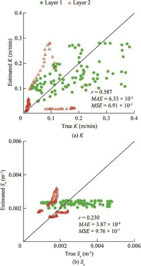
Fig.12.Comparison between true and estimated K and Ssfields using a highly parameterized inverse approach and head information in natural flow conditions.

Table 6Means and variances of true parameters of each layer of synthetic aquifer and those of estimated parameters for each layer based on different characterization approaches.

4.4.Highly parameterized approach with HT

Results of the numerical experiments described above encourage high-degree parameterization for an inverse problem.However，the resolution of estimates may not satisfy our needs and the estimate varies with different scenarios（Huang et al.，2011）.In order to accurately identify hydraulic properties of every element of the synthetic aquifer，previous discussions suggest that heads at at least three different times must be specified for every element of the solution domain and boundary fluxes must be known.This requirement is practically impossible to meet for any real world problem.As a consequence，finding ways of improving the resolution of the estimate with minimum additional effort and cost becomes an important task.Data fusion seems to be the answer.

The goal of data fusion is to synthesize data carrying nonredundant information about the heterogeneity in order to enhance the estimate of the heterogeneity.As discussed previously，the head at an observation well during the late times of a pumping test reflects heterogeneity everywhere within the cone of depression，but it is heavily influenced by the transmissivity near the observation and the pumping well.Such a finding implies that the head observed at one location during a pumping test likely carries information about heterogeneity difference from the head observed at the other locations（i.e.，non-redundant information）.By the same token，the heads observed at the same location that change due to pumping at different locations contain non-redundant information about heterogeneity within the cone of depression.Therefore，inclusion of head data from different pumping tests into estimations with a highly parameterized conceptual model will reveal more detailed heterogeneity and reduce the scenario dependence of the estimate.This is the foundation of the recently developed hydrologic data fusion technology，HT（Tosaka et al.，1993；Gottlieb and Dietrich，1995；Vasco et al.，2000；Yeh and Liu，2000；Bohling et al.，2002；Brauchler et al.，2003；Zhu and Yeh，2005，2006；Li et al.，2007；Liu et al.，2007；Illman et al.，2007，2008；Fienen et al.，2008；Ni et al.，2009；Castagna and Bellin，2009；Cardiff et al.，2009；Yin and Illman，2009；Illman et al.，2010）.

To illustrate utility of data fusion，an HT survey was simulated in thissynthetic aquifer.Itinvolved three independent pumping tests with a rate of 1 m3/min at nodes 1，3，and 11 in the aquifer（Fig.8（a））.Each pumping test started at a steady flow field corresponding to the boundary conditions of the previous natural flow case.During each pumping test at a given well，four temporal head measurements were recorded at the other 11 wells.Therefore，there were 132 head data available in total.These 132 head data，along with knowledge of the boundary conditions and an initial steady head distribution，were then used in SimSLE，a variant of SLE（Xiang et al.，2009），to estimate parameters K and Ss.Notice that previous examples，based on the sparsely and highly parameterized conceptual model，assumed a perfect knowledge of the initial head distribution during inversion.In this HT example，errors in the initial condition were introduced.Specifically，the initial head distribution was a simulated steady state head field based on the known boundary conditions and the estimated（not the true）K field from the previous natural flow scenario.An initial guess mean，variance，and correlation scale in the x and z directions for ln K（-3.0，2.0，50.0，and 3.0，respectively）and for ln Ss（-6.0，0.2，50.0，and 3.0，respectively）were used as input to SimSLE.

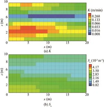
Fig.13.Estimates of K and Ssfields using a high-degree parameterization inverse approach.

Fig.14.Comparison between true and estimated K and Ssfields from a high-degree parameterization inverse approach and HT survey.

The estimated K and Ssfields are shown in Figs.13（a）and（b），respectively.Figs.14（a）and（b）show the corresponding scatter plots and the performance statistics.These figures indicate that HT yields better K and Ssestimates than those from the natural flow case，in general.

4.5.Validation

An ultimate goal of aquifer characterization is to improve predictions of head evolution or flow field induced by future stresses in the aquifer.Therefore，we followed validation approaches by Liu et al.（2007），Xiang et al.（2009），and Illman et al.（2010）to test our preceding estimates.That is，the estimated K and Ssfields from the three approaches（i.e.，the sparsely parameterized approach or zonation approach；highly parameterized approach or natural flow approach；highly parameterized approach with HT，called HT approach for short）were evaluated in terms of their ability to predict head and velocity fields induced by a new pumping event.This pumping event took place at x=9 m，and z=3 m（the solid square in Fig.8（a）with a constant rate of 1 m3/min.This event was not used in any previous inverse modeling efforts and it qualifies as an independent test.

Figs.15（a），（b），and（c）show plots of the true head vs. predicted heads at all nodes of the aquifer based on zonation， natural flow，and HT 5 min（early time）after pumping. Meanwhile，the same plots at late time（20 min after pumping）are shown in Figs.15（d），（e），and（f）.

Comparisons of true and predicted velocity in the x and z directions（Vxand Vz）at every node of the aquifer at late times in corresponding cases are shown in Fig.16.Performance statistics are also shown in these figures.Based on these figures and performance statistics，the estimates based on the HT approach，even with some uncertainty in initial head，clearly outperform those based on the natural flow approach alone.As expected，the estimates based on the natural flow approach yielded a better prediction than the estimates from the zonation approach.Notice that the estimates based on the natural flow approach yielded a Vxslightly worse than the zonation approach according to the performance statistics.Slightly worse predicted Vxvalues in Layer 2 using the natural flow and HT approaches were attributed to their estimates near the top boundary of Layer 2.

Lastly，the estimated K and Ssfields from the three approaches were tested for their ability to predict total outflow under uniform flow conditions.In this test，we assumed that the aquifer had a uniform total head 100 m everywhere initially.At timeslaterthanzero，thetotalheadattheleft-sideboundarywas increased to 110 m，while upper and lower boundary conditions were impermeable.Predicted outflows as a function of time at the right-side constant head boundary using the estimated parametersfromthethreeapproacheswerecomparedwiththetrue outflow in Fig.17.Again，the estimates based on the HT approach yieldedthebestresult.Thetrueoutflowatsteady state is0.050m3，whilesimulatedoutflowsusingKandSsfieldsfrom HT，zonation，and natural flow approaches are 0.051 m3，0.056 m3，and 0.048 m3，respectively.

In fact，using sandbox experiments，Liu et al.（2002，2007），Xiang et al.（2009），and Illman et al.（2010）have also substantiated the robustness of the estimates using HT and SLE，where model and measurement errors exist and are unknown. Likewise，Yeh and Zhu（2007）have demonstrated the power of hydraulic/tracer tomographic surveys with a highly parameterized model for mapping dense non-aqueous phase liquids（DNAPLS）.After all，a highly parameterized approach is not necessarily a setback to the inverse modeling.Furthermore，the improvement of the estimate throughout the aquifer by data fusion in a tomographic fashion suggests that head measurement in any part of an aquifer is always useful in spite of its low sensitivity.

5.Discussion and conclusions

The uniqueness issue of a real-world groundwater inverse problem stems from a lack of data satisfying the necessary conditions for defining the problem well.Effects of noise in the head，the unstable nature of the problem，and sensitivity are issues related to solution techniques.The necessary conditions for an inverse model to be well defined are a full specification of（1）flux boundaries or sources/sinks and（2）heads everywhere in the domain at at least three times（one of which is t=0）.

Fig.15.Comparison of predicted and observed heads at times of 5.0 min and 20.0 min during an independent pumping test for validating estimated parameters derived from different approaches.

A sparsely parameterized problem（such as a problem using few homogeneous zones）can be mathematically well defined. However，it may yield physically incorrect and phenomenological parameter values due to scale inconsistency between the scale of the head observation and REV concept embedded in the conceptual model.These problems can only be resolved by a sufficiently large number of spatial observations within each zone.

Using the same amount of data as in the zonation approach，a highly parameterized problem，even though it remains illdefined and perhaps suffers the same scale and scenariodependence issues，can lead to high-resolution maps of heterogeneity if it is solved properly.Furthermore，using the same pumping and monitoring facilities but interpreting data from several cross-holes，joint interference pumping tests（i.e.，HT） can yield results that improve our prediction of aquifer responses under different stresses.

Whilesimpleandhighlyparameterizedmodelshavebeenthe focusofmuchdiscussioninrecentyears（Hill，2006；Huntetal.，2007），we emphasize that the governing equations for flow through heterogeneous media strictly follow the principle of parsimony.Using the CV，the equations strip away complex movement of water molecules at molecular and pore scales that is not relevant at the scale of our interest and follows the principle of parsimony.Likewise，properly applied，highly parameterized approaches（such as the geostatistical and other regularization approaches）as well as HT are fully compliant withparsimonyattheincreasingresolutionsofourexamination.

Fig.16.Comparison of components of true and predicted velocity fields based on estimated parameters from different approaches at time of 20.0 min during independent pumping test.

The total outflow example also refutes a popular notion that water balance problems（or integrated metrics）do not require detailed K characterization（Haitjema，1995）.As shown in the example，detailed characterization yields more accurate accounting of total inflow，total change in storage，and total outflow.The key issue with the selection of a model is the resolution of our interest.A simple model always plays an important role since it provides a first-cut analysis of a complex system（Yeh，1992）.As the resolution of our interest increases，collecting more non-redundant data sets is the key to meet this demand.HT surveys are a cost-effective means for this purpose.Combination of HT data sets and a highly parameterized approach can enhance the resolution of aquifer characterization and，in turn，the accuracy of our predictions of groundwater flow.

Finally，we agree with Poeter and Hill（1997）and Carrera et al.（2005）that inverse modeling should become standard practice in hydrogeology.We also concur with Hunt et al.（2007）that high-degree parameterization may not be a bad strategy for inverse modeling if the inverse problem is solved properly.Finally，our results support the argument of changing the way we collect and analyze data，as suggested by Yeh andLee（2007）and the view of future subsurface characterization advocated by Yeh et al.（2008）.

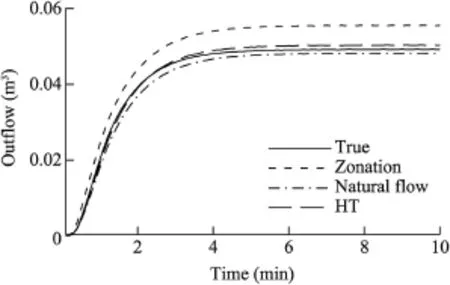
Fig.17.Comparison of true total outflow of synthetic aquifer and outflows predicted using zonation，natural flow，and HT approaches.

Acknowledgements

The first author acknowledges the Outstanding Oversea Professorship Award through Jilin University from the Department of Education in China.The second and the third authors acknowledge the support of the China Scholarship Council，in China.Finally，we thank Randy Hunt，Alec Desbarats，and Alberto Guadagnini for their constructive comments and suggestions，which significantly improved the quality of this paper.

References

Bear，J.，1972.Dynamics of Fluids in Porous Media.American Elsevier Publishing Company，Inc.，New York.

Bohling，G.C.，Zhan，X.Y.，Butler Jr.，J.J.，Zheng，L.，2002.Steady shape analysis of tomographic pumping tests for characterization of aquifer heterogeneities.Water Resour.Res.38（12），60-1-60-15.http://dx.doi.org/ 10.1029/2001WR001176.

Brauchler，R.，Liedl，R.，Dietrich，P.，2003.A travel time based hydraulic tomographic approach.Water Resour.Res.39（12）.http://dx.doi.org/ 10.1029/2003.WR002262.

Cardiff，M.，Barrash，W.，Kitanidis，P.K.，Malama，B.，Revil，A.，Straface，S.，Rizzo，E.，2009.A potential-based inversion of unconfined steady-state hydraulic tomography.Groundwater 47（2），259-270.http://dx.doi.org/ 10.1111/j.1745-6584.2010.00685_1.x.

Carrera，J.，Neuman，S.P.，1986.Estimation of aquifer parameters under transient and steady state conditions:2.Uniqueness，stability，and solution algorithms.Water Resour.Res.22（2），211-227.http://dx.doi.org/10.1029/ WR022i002p00199.

Carrera，J.，Alcolea，A.，Medina，A.，Hildalgo，J.，Slooten，L.，2005.Inverse problem in hydrogeology.J.Hydrol.13（1），206-222.http://dx.doi.org/ 10.1007/s10040-004-0404-7.

Castagna，M.，Bellin，A.，2009.A Bayesian approach for inversion of hydraulic tomographic data.Water Resour.Res.45（4），W04410.http:// dx.doi.org/10.1029/2008WR007078.

Dagan，G.，1982.Stochastic modeling of groundwater flow by unconditional and conditional probabilities:1.Conditional simulation and the direct problem.Water Resour.Res.8（4），813-833.http://dx.doi.org/10.1029/ WR018i004p00813.

Delhomme，J.P.，1979.Spatial variability and uncertainty in groundwater flow parameters:A geostatistical approach.Water Resour.Res.5（2），269-280. http://dx.doi.org/10.1029/WR015i002p00269.

de Marsily，G.，Lavedan，G.，Boucher，M.，Fasanino，G.，1984.Interpretation of interference tests in a well field using geostatistical techniques to fit the permeability distribution in a reservoir model.In:Verly，G.，David，M.，Journel，A.G.，Marechal，A.Eds.，Geostatistics for Natural Resources Characterization，Proceedings of the NATO Advanced Study Institute.D. Reidel Publishing Company，Dordrecht，pp.831-849.

de Marsily，G.，1986.Quantitative Hydrogeology:Groundwater Hydrology for Engineers.Academic Press，San Diego.

Doherty，J.，Hunt，R.J.，2009.Two statistics for evaluating parameter identifiability and error reduction.J.Hydrol.366（1-4），119-127.http:// dx.doi.org/10.1016/j.jhydrol.2008.12.018.

Doherty，J.，2010.PEST-ASP User'sManual.Watermark Numerical Computing，Brisbande.

Doherty，J.，Hunt，R.J.，2010.Reply to comment on:Two statistics for evaluating parameter identifiability and error reduction.J.Hydrol.380（3-4），489-496.http://dx.doi.org/10.1016/j.jhydrol.2009.10.012.

Emsellem，Y.，de Marsily，G.，1971.An automatic solution for the inverse problem.Water Resour.Res.7（5），1264-1283.http://dx.doi.org/10.1029/ WR007i005p01264.

Eppstein，M.J.，Dougherty，D.E.，1996.Simultaneous estimation of transmissivity values and zonation.Water Resour.Res.32（11），3321-3336. http://dx.doi.org/10.1029/96WR02283.

Fienen，M.N.，Clemo，T.，Kitanidis，P.K.，2008.An interactive Bayesian geostatistical inverse protocol for hydraulic tomography.Water Resour. Res.44（12），W00B01.http://dx.doi.org/10.1029/2007WR006730.

Frind，E.O.，Pinder，G.F.，1973.Galerkin solution of the inverse problem for aquifer transmissivity.Water Resour.Res.9（5），1397-1410.http:// dx.doi.org/10.1029/WR009i005p01397.

Gelhar，L.W.，1993.Stochastic Subsurface Hydrology.Prentice Hall，Upper Saddle River.

Gomez-Hernanez，J.，Sahuquillo，A.，Capilla，J.E.，1997.Stochastic simulation of transmissivity fields conditional to both transmissivity and piezometric data:1.Theory.J.Hydrol.204（1-4），162-174.http://dx.doi.org/10.1016/ S0022-1694（97）00098-x.

Gottlieb，J.，Dietrich，P.，1995.Identification of the permeability distribution in soil by hydraulic tomography.Inverse Probl.11（2），353-360.http:// dx.doi.org/10.1088/0266-5611/11/2/005.

Graham，W.，McLaughlin，D.，1989.Stochastic analysis of nonstationary subsurface solute transport:2.Conditional moments.Water Resour.Res. 25（11），2331-2355.http://dx.doi.org/10.1029/WR025i011p02331.

Hadamard，J.，1902.Sur les probl‵emes aux d′eriv′ees partielles et leur signification physique.Princeton University Bulletin 13，pp.49-52.

Haitjema，H.M.，1995.Analytic Element Modeling of Groundwater Flow. Academic Press，San Diego.

Hanna，S.，Yeh，T.-C.J.，1998.Estimation of co-conditional moments of transmissivity，hydraulic head，and velocity fields.Adv.Water Resour. 22（1），87-93.http://dx.doi.org/10.1016/S0309-1708（97）00033-X.

Harter，T.，Yeh，T.-C.J.，1996.Conditional stochastic analysis of solute transport in heterogeneous，variably saturated soils.Water Resour.Res. 32（6），1597-1609.http://dx.doi.org/10.1029/96WR00503.

Hill，M.C.，2006.The practical use of simplicity in developing ground water models.Groundwater 44（6），775-781.http://dx.doi.org/10.1111/j.1745-6584.2006.00227.x.

Hill，M.C.，2010.Comment on“Two statistics for evaluating parameter identifiabilityanderrorreduction”byJohnDohertyandRandallJ.Hunt.J.Hydrol. 380（3-4），481-488.http://dx.doi.org/10.1016/j.jhydrol.2009.10.011.

Huang，S.-Y.，Wen，J.-C.，Yeh，T.-C.J.，Lu，W.，Juan，H.-L.，Tseng，C.-M.，Lee，J.-H.，Chang，K.-C.，2011.Robustness of joint interpretation of sequential pumping tests:numerical and field experiments.Water Resour. Res.47，W10530.http://dx.doi.org/10.1029/2011WR010698.

Hughson，D.L.，Yeh，T.-C.J.，2000.An inverse model for three-dimensional flow in variably saturated porous media.Water Resour.Res.36（4），829-839.http://dx.doi.org/10.1029/2000WR900001.

Hunt，R.J.，Doherty，J.E.，Tonkin，M.J.，2007.Are models too simple？Arguments for increased parameterization.Groundwater 45（3），254-262. http://dx.doi.org/10.1111/j.1745-6584.2007.00316.x.

Illman，W.A.，Liu，X.，Craig，A.，2007.Steady-state hydraulic tomography in a laboratory aquifer with deterministic heterogeneity:Multi-method and multiscale validation of hydraulic conductivity tomograms.J.Hydrol. 341（3-4），222-234.http://dx.doi.org/10.1016/j.jhydrol.2007.05.011.

Illman，W.A.，Craig，A.J.，Liu，X.，2008.Practical issues in imaging hydraulic conductivity through hydraulic tomography.Groundwater 46（1），120-132. http://dx.doi.org/10.1111/j.1745-6584.2007.00374.x.

Illman，W.A.，Zhu，J.，Craig，A.J.，Yin，D.，2010.Comparison of aquifer characterization approaches through steady-state groundwater model validation:A controlled laboratory sandbox study.Water Resour.Res. 46（4）.http://dx.doi.org/10.1029/2009WR007745.

Indelman，P.，2003.Transient pumping well flow in weakly heterogeneous formations.Water Resour.Res.39（10），1287.http://dx.doi.org/10.1029/ 2003WR002036.

Jang，C.-S.，Liu，C.-W.，2004.Geostatistical analysis and conditional simulation for estimating the spatial variability of hydraulic conductivity in the Choushui River alluvial fan，Taiwan.Hydrol.Process.18（7），1333-1350. http://dx.doi.org/10.1002/hyp.1397.

Kitanidis，P.K.，1995.Quasi-linear geostatistical theory for inversing. WaterResour.Res.31（10），2411-2419.http://dx.doi.org/10.1029/ 95WR01945.

Knopman，D.，Voss，C.，1988.Discrimination among one-dimensional models of solute transport in porous media:Implications for sampling design. WaterResour.Res.24（11），1859-1876.http://dx.doi.org/10.1029/ WR024i011p01859.

Li，B.，Yeh，T.-C.J.，1999.Cokriging estimation of the conductivity field under variably saturated flow conditions.Water Resour.Res.35（12），3663-3674. http://dx.doi.org/10.1029/1999WR900268.

Li，W.，Englert，A.，Cirpka，O.A.，Vanderborght，J.，Vereecken，H.，2007.Two dimensional characterization of hydraulic heterogeneity by multiple pumping tests.Water Resour.Res.43（4），W04433.http://dx.doi.org/ 10.1029/2006WR005333.

Liu，S.，Yeh，T.-C.J.，Gardiner，R.，2002.Effectiveness of hydraulic tomography:Sandbox experiments.Water Resour.Res.38（4），5-1-5-9.http:// dx.doi.org/10.1029/2001WR000338.

Liu，X.，Illman，W.A.，Craig，A.J.，Zhu，J.，Yeh，T.-C.J.，2007.Laboratory sandbox validation of transient hydraulic tomography.Water Resour.Res. 43（5），W05404.http://dx.doi.org/10.1029/2006WR005144.

Mao，D.Q.，Yeh，T.-C.J.，Wan，L.，Hsu，K.-C.，Lee，C.-H.，Wen，J.-C.，2013. Necessary conditions for inverse modeling of flow through variably saturated porous media.J.Hydrol.52，50-61.http://dx.doi.org/10.1016/ j.advwatres.2012.08.001.

McLaughlin，D.，Townley，L.R.，1996.A reassessment of the groundwater inverse problem.Water Resour.Res.32（5），1131-1161.http://dx.doi.org/ 10.1029/2006WR005144.

Nævdal，G.，Johnsen，L.M.，Aanonsen，S.I.，Vefring，E.H.，2003.Reservoir monitoring and continuous model updating using ensemble Kalman filter.Soc.Petroleum Eng.J.10（1），66-74.http://dx.doi.org/10.2118/ 84372-PA.

Nelson，R.W.，1960.In-place measurement of permeability in heterogeneous media:1.Theory of a proposed method.J.Geophys.Res.65（6），1753-1758.http://dx.doi.org/10.1029/JZ065i006p01753.

Neuman，S.P.，1973.Calibration of distributed parameter groundwater flow models viewed as a multiobjective decision process under uncertainty. Water Resour.Res.9（4）， 1006-1021.http://dx.doi.org/10.1029/ WR009i004p01006.

Ni，C.F.，Yeh，T.-C.J.，Chen，J.-S.，2009.Cost-effective hydraulic tomography surveys for predicting flow and transport in heterogeneous aquifers.Environ.Sci.Technol.43（10），3720-3727.http://dx.doi.org/10.1021/ es8024098.

Poeter，E.P.，Hill，M.C.，1997.Inverse models:A necessary next step in groundwater modeling.Groundwater 35（2），250-260.http://dx.doi.org/ 10.1111/j.1745-6584.1997.tb00082.x.

Press，W.H.，Teukolsky，S.A.，Vetterling，W.T.，Flannery，B.P.，1992.Numerical Recipes in Fortran.Cambridge University Press，New York.

Smith，L.，Schwartz，F.W.，1981a.Mass transport:2.Analysis of uncertainty in prediction.Water Resour.Res.17（2），351-369.http://dx.doi.org/10.1029/ WR017i002p00351.

Smith，L.，Schwartz，F.W.，1981b.Mass transport:3.Role of hydraulic conductivity data in prediction.Water Resour.Res.17（5），1463-1479.http:// dx.doi.org/10.1029/WR017i005p01463.

Stallman，R.W.，1956.Numerical analysis of regional water levels to define aquifer hydrology.Trans.Am.Geophys.Union 37（4），451-460.http:// dx.doi.org/10.1029/TR037i004p00451.

Straface，S.，Yeh，T.-C.J.，Zhu，J.，Troisi，S.，Lee，C.H.，2007.Sequential aquifer tests at a well field，Montalto Uffugo Scalo，Italy.Water Resour. Res.43（7），W07432.http://dx.doi.org/10.1029/2006WR005287.

Sun，N.-Z.，Yeh，W.W.-G.，1985.Identification of parameter structure in groundwater inverse problem.Water Resour.Res.21（6），869-883.http:// dx.doi.org/10.1029/WR021i006p00869.

Sun，R.，Yeh，T.-C.J.，Mao，D.，Jin，M.，Lu，W.，Hao，Y.，2013.A temporal sampling strategy for hydraulic tomography analysis.Water Resour.Res. 49（7），3881-3896.http://dx.doi.org/10.1002/wrcr.20337.

Tosaka，H.，Masumoto，K.，Kojima，K.，1993.Hydropulse tomography for identifying 3-D permeability distribution.In:Proceedings of the 4th Annual International Conference on High Level Radioactive Waste Management.Amer Society of Civil Engineers，Las Vegas，pp.955-959.

Vasco，D.W.，Keers，H.，Karasaki，K.，2000.Estimation of reservoir properties using transient pressure data:An asymptotic approach.Water Resour.Res. 36（12），3447-3465.http://dx.doi.org/10.1029/2000WR900179.

Wagner，B.J.，Gorelick，S.M.，1989.Reliable aquifer remediation in the presence of spatially variable hydraulic conductivity:From data to design. WaterResour.Res.25（10），2211-2225.http://dx.doi.org/10.1029/ WR025i010p02211.

Wen，J.C.，Wu，C.M.，Yeh，T.-C.J.，Tseng，C.M.，2010.Estimation of effective aquifer hydraulic properties from an aquifer test with multi-well observations（Taiwan）.J.Hydrol.18（5），1143-1155.http://dx.doi.org/10.1007/ s10040-010-0577-1.

Wu，C.-M.，Yeh，T.-C.J.，Zhu，J.，Lee，T.H.，Hsu，N.-S.，Chen，C.-H.，Sancho，A.F.，2005.Traditional analysis of aquifer tests:Comparing apples to oranges？Water Resour.Res.41（9），W09402.http://dx.doi.org/10.1029/ 2004WR003717.

Xiang，J.，Yeh，T.-C.J.，Lee，C.-H.，Hsu，K.-C.，Wen，J.-C.，2009.A simultaneous successive linear estimator and a guide for hydraulic tomography analysis.Water Resour.Res.45（2），W02432.http://dx.doi.org/10.1029/ 2008WR007180.

Ye，M.，Khaleel，R.，Yeh，T.-C.J.，2005.Stochastic analysis of moisture plume dynamics of a field injection experiment.Water Resour.Res.41（3），W03013.http://dx.doi.org/10.1029/2004WR003735.

Yeh，T.-C.J.，Gelhar，L.W.，Gutjahr，A.L.，1985a.Stochastic analysis of unsaturated flow in heterogeneous soils:1.Statistically isotropic media. Water Resour.Res.21（4）， 447-456.http://dx.doi.org/10.1029/ WR021i004p00447.

Yeh，T.-C.J.，Gelhar，L.W.，Gutjahr，A.L.，1985b.Stochastic analysis of unsaturated flow in heterogeneous soils:2.Statistically anisotropic media. Water Resour.Res.21（4）， 457-464.http://dx.doi.org/10.1029/ WR021i004p.00457.

Yeh，T.-C.J.，Gelhar，L.W.，Gutjahr，A.L.，1985c.Stochastic analysis of unsaturated flow in heterogeneous soils:3.Observations and applications. Water Resour.Res.21（4）， 465-471.http://dx.doi.org/10.1029/ WR021i004p.00465.

Yeh，T.-C.J.，1992.Stochastic modeling of groundwater flow and solute transport in aquifers.Hydrol.Process.6（4），369-395.http://dx.doi.org/ 10.1002/hyp.3360060402.

Yeh，T.-C.J.，Srivastava，R.，Guzman，A.，Harter，T.，1993.A numerical model for two dimensional flow and chemical transport.Groundwater 31（4），634-644.

Yeh，T.-C.J.，Jin，M.，Hanna，S.，1996.An iterative stochastic inverse method:Conditional effective transmissivity and hydraulic head fields. Water Resour.Res.32（1）， 85-92.http://dx.doi.org/10.1029/ 95WR02869.

Yeh，T.-C.J.，Liu，S.，2000.Hydraulic tomography:Development of a new aquifer test method.Water Resour.Res.36（8），2095-2105.http:// dx.doi.org/10.1029/2000WR900114.

Yeh，T.-C.J.，Liu，S.，Glass，R.J.，Baker，K.，Brainard，J.R.，Alumbaugh，D.，LaBrecque，D.，2002.A geostatistically based inverse model for electrical resistivity surveys and its applications to vadose zone hydrology.Water Resour.Res.38（12），14-1-14-3.http://dx.doi.org/10.1029/2001WR001204.

Yeh，T.-C.J.，Ye，M.，Khaleel，R.，2005.Estimation of effective unsaturated hydraulic conductivity tensor using spatial moments of observed moisture plume.Water Resour.Res.41（3），W03014.http://dx.doi.org/10.1029/ 2004WR003736.

Yeh，T.-C.J.，Lee，C.H.，2007.Time to change the way we collect and analyze data for aquifer characterization.Groundwater 45（2），116-118.http:// dx.doi.org/10.1111/j.1745-6584.2006.00292.x.

Yeh，T.-C.J.，Zhu，J.，2007.Hydraulic/partitioning tracer tomography for characterization of dense nonaqueous phase liquid source zones.Water Resour.Res.43（6），W06435.http://dx.doi.org/10.1029/2006WR004877.

Yeh，T.-C.J.，Lee，C.H.，Hsu，K.C.，Illman，W.A.，Barrash，W.，Cai，X.，Daniels，J.，Sudicky，E.，Wan，L.，Li，G.，Winter，C.L.，2008.Aview toward the future of subsurface characterization:CAT scanning groundwater basins.Water Resour.Res.44（3），W03301.http://dx.doi.org/10.1029/ 2007WR006375.

Yin，D.，Illman，W.A.，2009.Hydraulic tomography using temporal moments of drawdown recovery data:A laboratory sandbox study.Water Resour. Res.45（1），W01502.http://dx.doi.org/10.1029/2007WR006623.

Zimmerman，D.A.，deMarsily，G.，Gotway，C.A.，Marietta，M.G.，Axness，C.L.，Beauheim，R.L.，Bras，R.L.，Carrera，J.，Dagan，G.，Davies，P.B.，Gallegos，D.P.，1998.A comparison of seven geostatistically based inverse approaches to estimate transmissivities for modeling advective transport by groundwater flow.Water Resour.Res.34（6），1373-1413.http://dx.doi.org/10.1029/98WR00003.

Zhang，J.，Yeh，T.-C.J.，1997.An iterative geostatistical inverse method for steady flow in the vadose zone.Water Resour.Res.33（1），63-71.http:// dx.doi.org/10.1029/96WR02589.

Zhu，J.，Yeh，T.-C.J.，2005.Characterization of aquifer heterogeneity using transient hydraulic tomography.Water Resour.Res.41（7），W07028.http:// dx.doi.org/10.1029/2004WR003790.

Zhu，J.，Yeh，T.-C.J.，2006.Analysis of hydraulic tomography using temporal moments of drawdown-recovery data.Water Resour.Res.42（2），W02403. http://dx.doi.org/10.1029/2005WR004309.

Zhu，J.，Cai，X.，Yeh，T.-C.J.，2009.Analysis of tracer tomography using temporal moments of tracer breakthrough curves.Adv.Water Resour. 32（3），391-400.http://dx.doi.org/10.1016/j.advwatres.2008.12.001.

This work was supported by the Strategic Environmental Research and Development Program（Grant No.ER-1365），the Environmental Security and Technology Certification Program（Grant No.ER201212），and the Earth Sciences of the National Science Foundation（Grant No.1014594）.

*Corresponding author.

E-mail address:ybiem@mac.hwr.arizona.edu（Tian-chyi J.Yeh）.

Peer review under responsibility of Hohai University.

http://dx.doi.org/10.1016/j.wse.2015.08.002

1674-2370/©2015 Hohai University.Production and hosting by Elsevier B.V.This is an open access article under the CC BY-NC-ND license（http:// creativecommons.org/licenses/by-nc-nd/4.0/）.