A TVD-WAF-based hybrid finite volume and finite difference scheme for nonlinearly dispersive wave equations

Jing Yin*，Jia-wen SunZi-feng Jiao

aNational Marine Environment Monitoring Center，State Oceanic Administration，Dalian 116023，PR China

bState Key Laboratory of Coastal and Offshore Engineering，Dalian University of Technology，Dalian 116024，PR China

Received 22 October 2014；accepted 23 June 2015

Available online 15 August 2015

A TVD-WAF-based hybrid finite volume and finite difference scheme for nonlinearly dispersive wave equations

Jing Yina，b，*，Jia-wen Suna，b，Zi-feng Jiaob

aNational Marine Environment Monitoring Center，State Oceanic Administration，Dalian 116023，PR China

bState Key Laboratory of Coastal and Offshore Engineering，Dalian University of Technology，Dalian 116024，PR China

Received 22 October 2014；accepted 23 June 2015

Available online 15 August 2015

Abstract

A total variation diminishing-weighted average flux（TVD-WAF）-based hybrid numerical scheme for the enhanced version of nonlinearly dispersive Boussinesq-type equations was developed.The one-dimensional governing equations were rewritten in the conservative form and then discretized on a uniform grid.The finite volume method was used to discretize the flux term while the remaining terms were approximated with the finite difference method.The second-order TVD-WAF method was employed in conjunction with the Harten-Lax-van Leer（HLL）Riemann solver to calculate the numerical flux，and the variables at the cell interface for the local Riemann problem were reconstructed via the fourthorder monotone upstream-centered scheme for conservation laws（MUSCL）.The time marching scheme based on the third-order TVD Runge-Kutta method was used to obtain numerical solutions.The model was validated through a series of numerical tests，in which wave breaking and a moving shoreline were treated.The good agreement between the computed results，documented analytical solutions，and experimental data demonstrates the correct discretization of the governing equations and high accuracy of the proposed scheme，and also conforms the advantages of the proposed shock-capturing scheme for the enhanced version of the Boussinesq model，including the convenience in the treatment of wave breaking and moving shorelines and without the need for a numerical filter.

©2015 Hohai University.Production and hosting by Elsevier B.V.This is an open access article under the CC BY-NC-ND license（http:// creativecommons.org/licenses/by-nc-nd/4.0/）.

Hybrid scheme；Finite volume method（FVM）；Finite difference method（FDM）；Total variation diminishing-weighted average flux（TVD-WAF）；Boussinesq-type equations；Nonlinear shallow water equations（NSWEs）

1.Introduction

Due to the complexity and computation expense required to solve the full Navier-Stokes equations in numerical modeling of free surface flows，a depth-averaged assumption is employed in some cases to simplify the problem by neglecting the vertical component of the momentum equations.Nonlinear shallow waterequations（NSWEs）andBoussinesq-type equations are the most representative and well known depthaveraged models.

NSWEs are usually used to solve the flow motion in rivers，lakes，and tide bores.A high-resolution numerical scheme using the finite volume method（FVM）has been developed to solve NSWEs and has shown agreement with analytical solutions and experimental and field data（Toro，2009；Hubbard and Dodd，2002；Liang et al.，2008）.In addition to its ability to deal with irregular boundaries using unstructured grids，the FVM-type discretization of NSWEs has another two merits:a shock-capturing ability and its treatment of the moving shoreline as a local Riemann problem（Toro，2009）.Unfortunately，NSWEs fail to model dispersive wave propagation，because，in deeper water，dispersion has an effect on freesurface flow.Boussinesq-type equations，in contrast，are more applicable to describing dispersive and nonlinear waves in coastal regions（Madsen and Fuhrman，2010）.

The finite difference method（FDM）is most widely used for numerical solution of Boussinesq-type equations（Madsen and Fuhrman，2010；Gobbi et al.，2000；Lynett，2006；Fuhrman and Madsen，2008；Fang et al.，2014），although there are examples of the finite element method（FEM）（Sørensen et al.，2004）and FVM （Shi et al.，2012）.The FDM-based Boussinesq-type models have achieved great success and have been widely used to simulate wave transformation from deep water to swash zonesand wave-induced currents（Madsen and Fuhrman，2010）.However，researchers have recognized the defects of FDM in solving Boussinesq-type equations.First，models have proven to be noisy，and the periodic use of a numerical filter is required to stabilize the model；Second，wave breaking and moving shorelines are only approximated via the ad-hoc method in Boussinesq-type models（e.g.，the artificial viscosity method for wave breaking and the slot method for moving shorelines），which introduces an additional source of noise and causes more uncertainty，since many tunable parameters are involved（Madsen and Fuhrman，2010；Gobbi et al.，2000；Lynett，2006；Fuhrman and Madsen，2008；Shi et al.，2012）.

In recognition of the fact that NSWEs are an intrinsic part of Boussinesq-type equations，researchers have attempted to solve Boussinesq-type equations using a hybrid method combining FVM and FDM（Shi et al.，2012；Erduran，2007；Tonelli and Petti，2009；Orszaghova et al.，2012；Cienfuegos et al.，2007；Shiach and Mingham，2009；Roeber et al.，2010）.The resulting hybrid models have shown robust performance.In particular，the models are quite stable，and the additional filter is no longer required.In addition，by switching off the dispersive terms at a local scale，Boussinesq-type equations revert to NSWEs，wave breaking is approximated as shock waves，and the moving shoreline is treated as a discontinuity，which is accepted by NSWEs.In this way，the drawbacks of FDM-based Boussinesq-type equations are remedied，and a more efficient coastal wave model can be obtained.

Existing hybrid approaches use the first-order monotone flux，usually，the Harten-Lax-van Leer（HLL）-type function，to calculate the numerical flux through the cell interface，which may not be an accurate enough method of capturing the relatively sharp waves，for example，breaking waves and highly nonlinear waves.Actually，the accuracy of the highorder flux over the first-order flux has already been proven for a hyperbolic system，for example，NSWEs.It is therefore straightforward to use a high-order flux method to develop the hybrid FVM/FDM scheme for Boussinesq-type equations.In this study，we used the second-order total variation diminishing-weighted average flux（TVD-WAF）method to develop a shock-capturing scheme for the Boussinesq model. The novel hybrid scheme was then applied to solution of a setof weakly dispersive and nonlinearly dispersive Boussinesq-type equations derived by Kim et al.（2009）.

2.Mathematical model

2.1.Boussinesq-type equations for rapidly varying bathymetry

Kim et al.（2009）presented an enhanced version of Madsen and Sorensen's Boussinesq equations，which has the forms of

where η is the surface elevation；d is the total water depth，and d=h+η，where h is the still water depth；q is the volume flux，and q=du，where u is the depth-averaged flow velocity in the x direction；g is the gravitational acceleration；and

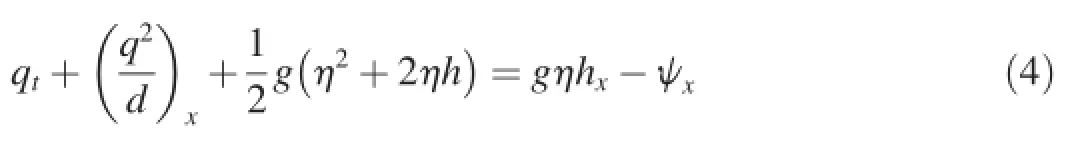
The subscripts x and t denote the partial derivatives with respect to the x direction and time，respectively，and B is a tunable parameterused fordispersion.The Pad′e［2，2］approximation of the linear dispersion relation is obtained by setting B=1/15.By neglecting high-order terms related to the seabed（the last two terms in Eq.（3））under the assumption of a mild slope，the equations revert to Madsen and Sorensen's Boussinesq equations（Madsen and Sørensen，1992）.However，including these terms helps to improve the model's performance with regard to rapidly varying bathymetry（Kim et al.，2009）.To facilitate the FVM discretization，the term gdηxis rearranged as g（η2+2ηh）/2-gηhx，and Eq.（2）becomes

2.2.Conservative form of Boussinesq-type equations

The generalized conservative form of Boussinesq-type equations can be written as

where U and F（U）are vectors containing the conserved variables and fluxes，respectively，and S is the vector of source terms:

where

R denotes the bottom friction and is formulated as R=cfu|u|，where cfis the friction coefficient，with a default value of zero unless a certain value is assigned.

2.3.Equation discretization

The computation domain is discretized into N grid cells with xi=iΔx（i=1，2，…，N）.Integrating the governing equations for the ith grid cell over the bounded range［xi-1/2，xi+1/2］and time duration Δt and using Green's theorem lead to

2.4.Calculation of numerical flux and remaining terms

A hybrid method combing FVM and FDM is used for spatial discretization.The main procedure for FVM implementation is calculation of the numerical flux in Eq.（9）. Numerous schemes can be used for this（Toro，2009）.Previous hybrid approaches for Boussinesq-type equations used the first-order monotone numerical flux.In this study，we used the second-order TVD-WAF method.

The WAF method depends on the selection of an approximation for the intermediate waves，and the HLL Riemann solver is preferred as it better describes the flux for a dry-bed situation and does not require any entropy fix（Toro，2009）.In the HLL Riemann solver the numerical flux is approximated according to Toro（2009）:

where the subscripts L and R denote the variables with values on the left and right sides of a cell interface for a local Riemann problem，respectively.In order to apply the HLL Riemann solver to shallow water equations，it is important to identify the wave speeds SLand SRcorrectly.Toro（2009）recommended the use of a two-rarefaction approximate Riemann solver for SLand SR:

where

According to Yamamoto et al.（1998），a fourth-order monotone upstream-centered scheme for conservation laws（MUSCL）is used to reconstruct the vector U at the cell interface.

The WAF scheme is a fully explicit second-order（both in time and space）extension of the Godunov first-order upwind scheme.The basic idea of the WAF method is to define the numerical flux as a weighted average of the fluxes of different wave components in the solution of the local Riemann problem at a half time step:

where F′kis the kth flux corresponding to the kth wave component；K is the number of wave components，and for a one-dimensional problem K=2；and wkis the weight of the kth flux and is given by

where ckis the local Courant-Friedrichs-Lewy（CFL）number of the kth wave component，with

where Skis the speed of kth wave component.

Substituting Eq.（16）and Eq.（17）into Eq.（15），an alternative expression of the numerical flux at the right interface of the ith grid cell at the nth time step can be obtained:

The source term Siin Eq.（9）is approximated using the high-order FDM（Orszaghova et al.，2012），which is accurate enough to remove any false dispersion caused by truncation error.

2.5.Time marching scheme

The third-order TVD version of the Runge-Kutta scheme（Gottlieb et al.，2001）is adopted for time marching，which is given by

As the source term is approximated implicitly in the last step in Eq.（20），iteration is required to achieve the final solution.The iteration is stopped once the relative error of adjacent solutions is less than an allowed minimum，i.e.，1.0×10-4in these simulations.

The time step Δt is restricted by the following expression:

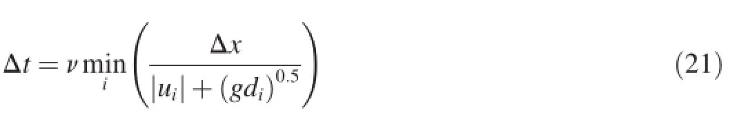
where ν is set to be 0.5 in the simulations，diis the water depth in cell i，and uiis the flow velocity in cell i.

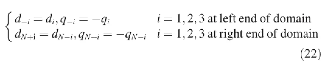
2.6.Boundary conditions and wave breaking

The entire computational domain is enclosed by impermeable walls，and three ghost cells are defined，with the values of the three cells being

Sponge layers are placed in front of solid walls to absorb wave energy，with the following modification function:

where xsis the length of the sponge layer，with a value of two times a typical wavelength.

Theincidentwavesareinternally generated in the computational domain by adding a source function to the mass equation（Gobbi et al.，2000）.According to Fang et al.（2013），the thin film method was adopted to deal with the wet-dry interface in this study.A critical water depth of 0.001 m was used to distinguish cells in the dry state（if d≤0.001 m）and in the wet state（if d＞0.001 m）.A cell with water depth less than or equal to the critical water depth was defined as a dry cell adjacent to a wet cell.The wet-dry interface was defined as the cell interface between wet and dry cells.In this manner the moving wet-dry interface was automatically captured.

In this study，Boussinesq equations reverted to NSWEs through switching off dispersive terms in the cells where the ratio of the surface elevation to water depth exceeded 0.80 and wave breaking occurred.According to Shi et al.（2012）and Fang et al.（2013），wave breaking was treated as a discontinuity and numerically described by NSWEs.

3.Numerical results and discussion

In order to demonstrate the capability of the hybrid model developed in this study，the model was used in several tests:（1）wave sloshing in a closed water tank，（2）sinusoidal wave propagation over deep water with a constant water depth，（3）a solitary wave traveling in a frictionless water channel with a flat bottom，（4）regular wave propagation over a submerged bar in a wave flume with a flat bottom，and（5）solitary wave breaking and runup over a sloping beach.The available experimental data and analytical solutions were used for model validation.It should be mentioned that no numerical filter was used for the simulations.

3.1.Wave sloshing in a closed water tank

In this test，water sloshing in a closed water tank was considered.The tank was 10 m long，and the still water depth h was 0.2 m.The free surface of fluid had an initial slope of s=0.0002，and the fluid was released and moved with the gravity.The analytical solution to the fluid motion could be found using the linear wave theory（Lin and Man，2007），neglecting the viscous and nonlinear effects.As the water was enclosed by solid walls，the mass needed to be unchanged during the calculation process.This test is therefore a good benchmark test for model validation.

In the numerical simulation，the domain was discretized into 200 uniform cells with a cell size Δx=0.05 m.The instantaneous surface elevations at t/T=0，0.2，0.4，0.6，0.8，1.0，3.0，4.0，and 5.0 are shown in Fig.1，where T is the wave period of the leading mode of the standing wave，with T=14.2 s in this study.During the first wave period，where t/T≤ 1，the computed results agree with the analytical solutions，and the overall agreements for a long simulation（t/T=3，4，and 5）remain fairly good，implying that both the mass and wave energy are conserved during the numerical computation.In Fig.2，we present the time history of water mass（M）in the water tank during an even longer simulation time，i.e.，500 s，with a fluctuation of less than 0.1%，demonstrating the high accuracy of this hybrid scheme.

Fig.1.Comparison of simulated free surface elevations and analytical solutions at different instants in closed water tank.

Fig.2.Time series of water mass during simulation（M0is initial water mass in water tank）.

3.2.Regular wave propagation over deep water with constant depth

The second test was the sinusoidal wave propagation over deep water with a horizontal bottom.The wave tank was 200 m long，and the still water depth h was 4.2 m.The incident regular wave had a period of T=2.5 s and an amplitude of A=0.1 m.In this case，the ratio of the still water depth to wavelength h/L0was 0.43，close to the deep water limit，i.e.，h/L0=0.5，and also within the applicable range of the equations.In the numerical simulation，the wave tank was discretized into 1000 uniform cells，and waves were then generated in the middle of the tank.Two sponge layers，with widths of 20 m，were placed at the two ends of the wave tank to absorb wave energy.

The incoming waves were generated by the internal source and well developed in the wave tank.The simulated free surface elevations at four different instants are plotted in Fig.3，demonstrating the effectiveness of the sponge layer at the two ends of the wave tank.The model was then run for the second time by removing the sponge layer at the right end of the tank.The corresponding computed free surface elevations are also plotted in Fig.3.The computed results of the first two instants are identical to those of the first run.However，the standing wave pattern occurs once the right-going waves encounter the right solid wall，as shown in Figs.3（f）and（h）. Finally the whole domain is occupied by standing waves，with the amplitude reaching two times that of the initial incident waves.The effectiveness of the sponge layer is again shown at the left end of the wave tank by the present hybrid scheme.

3.3.Solitary wave propagation over flat bottom

Numerical simulation of solitary wave propagation over a long frictionless channel with a constant still water depth is a common test for numerical models（Zhang et al.，2015）.The solitary wave is characterized by a single symmetric pulse above the still water level，propagating at a constant velocity. The wave shape remains unchanged due to the exact balance between dispersion and nonlinearity.Any improper numerical treatment will lead to poor balance and finally spoil the wave shape.

A solitary wave with an amplitude of A=0.6 m，propagating in still water with a still water depth of h=1.0 m，was simulated using the present hybrid model.The channel was 375 m long，and the cell size Δx was 0.05 m.According to the procedure of Orszaghova et al.（2012），the analytical solutions of the solitary wave to Eq.（1）and Eq.（2）could be obtained and taken as the initial condition of the model（an initial crest center at x=50 m）.The computed solitary wave profiles at eight instants are plotted in Fig.4.The wave shape remains unchanged during the propagation，confirming that the governing equations were discretized correctly，and that the time marching scheme performed well during the numerical simulation.In Fig.5，the computed wave profile at the instant t=70 s is compared with the analytical solution.They are in excellent agreement，demonstrating the model's ability to correctly predict wave speed.

Fig.3.Computed surface elevations under non-reflective boundary and fully reflective right boundary at four instants.

Fig.4.Computed solitary wave profiles at different instants.

Fig.5.Comparison of numerical and analytical results of solitary wave profiles at t=70 s.

3.4.Regular wave propagation over submerged bar

It is well known that regular wave propagation over a submerged bar is an extremely complicated process:nonlinear interactions transfer energy from the leading wave component to higher harmonics as waves propagate to the front slope of the bar，and waves thus steepen.At the leeside of the bar，the water depth increases，and the nonlinear coupling of the higher harmonics with the fundamental wave progressively weakens. These harmonics travel at different speeds，causing a fairly complicated process.Numerical prediction of this process requires a model with higher-order linear and nonlinearaccuracy，and it has been widely utilized as a benchmark test for validating Boussinesq-type models（Gobbi et al.，2000）.

Case（a）in experiments of Luth et al.（1994）was simulated，and the corresponding experimental setup is shown in Fig.6. The wave flume was 23 m long.In a wave flume with a still water depth of h=0.4 m，a trapezoidal bar with an upward slope of 1:20 and a steeper downward slope of 1:10 was created.The minimum water depth on the bar top was 0.1 m. A sinusoidal wave with a period of T=2.02 s and a wave height of H=0.02 m was generated in the computational domain.

The numerical simulation was performed with the cell size Δx=0.02 m.The numerical results of free surface elevations at locations x=2.0，5.7，10.5，13.5，15.7，and 19.0 m are given in Fig.7，and are compared with the experimental data.The numerical results are in good agreement with those measured on the upward slope and on the bar top.It should be noted that the phase discrepancy at x=5.7 m is attributed to an error in the record of the experiments（Shiach and Mingham，2009）. However the numerical model fails to predict the wave shape on the downward slope，especially at x=19.0 m behind the bar.The discrepancies are mainly caused by the weak dispersion of the governing equations（Madsen and Sørensen，1992；Erduran，2007）.The numerical results from Shiach and Mingham（2009）using Madsen and Sørensen's Boussinesq equations are also plotted for comparison.At the first three locations，the numerical results from two models are primarily the same，while the difference occurs on the bar top and behind the bar.It is hard to say which one is better，and the difference is mainly caused by different numerical schemes. We also neglected the high-order bottom slope terms in Eq.（3）in another run of this model，and no difference was found.It is expected that the higher-order derivative hxxis equal to zero andis at low values in this case.

Fig.6.Experimental setup in Luth et al.（1994）

Fig.7.Comparison of computed free surface elevations with experimental data.

3.5.Solitary wave breaking and runup on sloping beach

In order to test the model's ability to simulate wave breaking and runup，we conducted the numerical test for solitary wave breaking and runup on a sloping beach and compared the numerical results with experimental data from Synolakis（1987）.The beach had a slope of 1:19.85，and the still water depth h over the flat bottom was 0.39 m，as shown Fig.8.

In the simulation，the analytical form of the initial solitary wavewas specified as the initial condition in the computational domain.One of the cases for a solitary wave in Synolakis（1987），with a dimensionless wave height H/h=0.3，was selected for simulation.The computational domain was 30 m long and discretized using the cell size Δx=0.02 m.The bed friction coefficient cfwas 0.001.For the sake of convenience，the computed results were non-dimensionalized as x*=x/h，η*=η/h，and t*=t（g/h）0.5.

The computed surface elevations at the different instants t*=15，20，25，and 30 were compared with experimental data，as shown in Fig.9.The wave shoaling occurs and the front face becomes steep at t*=15（Fig.9（a））.At t*=20，wave breaking occurs，and the model captures it as a shock with an almost a vertical wave front（Fig.9（b））.The breaking wave then propagates onto the beach，resulting in wave runup at t*=20 and 30.These phenomena are well reproduced by the present model，indicating that the model captures shoaling，wave breaking，and moving shorelines efficiently.However，the computed wave crest in Fig.9（b）is slightly underestimated by the model，indicating that the present model tends to predict an earlier breaking event.This is consistent with Fang et al.（2015），where the same breaking criterion was employed in the same test.

4.Conclusions

（1）A TVD-WAF-based hybrid finite volume and finite difference scheme was proposed to solve the enhanced version of the Boussinesq equations.The flux terms were discretized using FVM while the rest terms are treated using FDM.A second-order TVD-WAF scheme，instead of the commonly used HLL scheme，was adopted in conjunction with the MUSCL method to compute the numerical flux.Wave breaking and moving shorelines were also treated with the model.

Fig.8.Sketch of solitary wave runup on a sloping beach.

Fig.9.Runup of breaking solitary wave with H/h=0.3 on sloping beach at different non-dimensional instants.

（2）Numerical tests were conducted for model validation. The good agreement between the computed results and analytical solutions demonstrates the correct discretization of the governing equations，the high accuracy of the proposed scheme，and the efficient treatment of the non-reflective wave generation.The successful simulation of dispersive wave propagation over a submerged bar and solitary wave breaking and runup over a sloping beach further confirms the advantages of the proposed shock-capturing scheme for the enhanced version of the Boussinesq model，including the convenience in the treatment of wave breaking and moving shorelines and without the need for a numerical filter.

References

Cienfuegos，R.，Barth′elemy，E.，Bonneton，P.，2007.A fourth-order compact finitevolume scheme forfully nonlinearand weakly dispersive Boussinesq-type equations，part II:Boundary conditions and validation. Int.J.Numer.Methods Fluids 53（9），1423-1455.http://dx.doi.org/ 10.1002/fld.1359.

Erduran，K.S.，2007.Further application of hybrid solution to another form of Boussinesq equations and comparisons.Int.J.Numer.Methods Fluids 53（5），827-849.http://dx.doi.org/10.1002/fld.1307.

Fang，K.Z.，Zou，Z.L.，Dong，P.，Liu，Z.B.，Gui，Q.Q.，Yin，J.W.，2013.An efficient shock capturing algorithm to the extended Boussinesq wave equations.Appl.Ocean Res.43，11-20.http://dx.doi.org/10.1016/ j.apor.2013.07.001.

Fang，K.Z.，Yin，J.W.，Liu，Z.B.，Sun，J.W.，Zou，Z.L.，2014.Revisiting study on Boussinesq modeling of wave transformation over various reef profiles. Water Sci.Eng.7（3），306-318.http://dx.doi.org/10.3882/j.issn.1674-2370.2014.03.006.

Fang，K.Z.，Liu，Z.B.，Zou，Z.L.，2015.Efficient computation of coastal waves using a depth-integrated，non-hydrostatic model.Coast.Eng.97，21-36. http://dx.doi.org/10.1016/j.coastaleng.2014.12.004.

Fuhrman，D.R.，Madsen，P.A.，2008.Simulation of nonlinear wave run-up with a high-order Boussinesq model.Coast.Eng.55（2），139-154.http:// dx.doi.org/10.1016/j.coastaleng.2007.09.006.

Gobbi，M.F.，Kirby，J.T.，Wei，G.，2000.A fully nonlinear Boussinesq model for surface waves，part 2:Extension to O（kh）4.J.Fluid Mech.405（4），181-210.http://dx.doi.org/10.1017/S0022112099007247.

Gottlieb，S.，Shu，C.W.，Tadmore，E.，2001.Strong stability-preserving highorder time discretization methods.SIAM Rev.43（1），89-112.http:// dx.doi.org/10.1137/S003614450036757X.

Hubbard，M.E.，Dodd，M.，2002.A 2D numerical model of wave run-up and overtopping.Coast.Eng.47（1），1-26.http://dx.doi.org/10.1016/s0378-3839（02）00094-7.

Kim，G.，Lee，C.，Suh，K.D.，2009.Extended Boussinesq equations for rapidly varying topography.Ocean Eng.36（11），842-851.http://dx.doi.org/ 10.1016/j.oceaneng.2009.05.002.

Liang，Q.，Du，G.Z.，Hall，J.W.，Borthwick，A.G.L.，2008.Flood inundation modeling with an adaptive quadtree grid shallow water equation solver.J. Hydraul.Eng.134（1），1603-1610.http://dx.doi.org/10.1061/（asce）0733-9429（2008）134:11（1603）.

Lin，P.，Man，C.，2007.A staggered-grid numerical algorithm for the extended Boussinesq equations.Appl.Math.Model.31（2），349-368.http:// dx.doi.org/10.1016/j.apm.2005.11.012.

Luth，H.R.，Klopman，G.，Kitou，N.，1994.Kinematics of Waves Breaking Partially on an Offshore Bar:LDV Measurements of Waves With and Without a Net Onshore Current（Report H-1573）.Delft Hydraulics，pp.40.

Lynett，P.J.，2006.Nearshore wave modeling with higher-order Boussinesqtype equations.J.Waterway Port Coast.Ocean Eng.132（5），348-357. http://dx.doi.org/10.1061/（asce）0733-950x（2006）132:5（348）.

Madsen，P.A.，Sørensen，O.R.，1992.A new form of the Boussinesq equations with improved linear dispersion characteristics，part 2:A slowly-varying bathymetry.Coast.Eng.18（3-4），183-204.http://dx.doi.org/10.1016/ 0378-3839（92）90019-q.

Madsen，P.A.，Fuhrman，D.R.，2010.High-order Boussinesq-type modeling of nonlinear wave phenomena in deep and shallow water.In:Ma，Q.，Ed.，Advances in Numerical Simulation of Nonlinear Water Waves.World Scientific Publishing Co.Pte.Ltd.，pp.245-285.http://dx.doi.org/10. 1142/9789812836502_0007.

Orszaghova，J.，Borthwick，A.G.L.，Taylor，P.H.，2012.From the paddle to the beach:A Boussinesq shallow water numerical wave tank based on Madsen and Sørensen's equations.J.Comput.Phys.231（2），328-344.http:// dx.doi.org/10.1016/j.jcp.2011.08.028.

Roeber，V.，Cheung，K.F.，Kobayashi，M.H.，2010.Shock-capturing Boussinesq-type model for nearshore wave processes.Coast.Eng.57（4），407-423.http://dx.doi.org/10.1016/j.coastaleng.2009.11.007.

Shi，F.Y.，Kirby，J.T.，Harris，J.C.，Geiman，J.D.，Grilli，S.T.，2012.A higherorder adaptive time-stepping TVD solver for Boussinesq modeling of breaking waves and coastal inundation.Ocean Model.43（44），36-51. http://dx.doi.org/10.1016/j.ocemod.2011.12.004.

Shiach，J.B.，Mingham，C.G.，2009.A temporally second-order accurate Godunov-typeschemefor solvingthe extendedBoussinesqequations.Coast. Eng.56（1），32-45.http://dx.doi.org/10.1016/j.coastaleng.2008.06.006.

Sørensen，O.R.，Schaffer，H.A.，Sørensen，L.S.，2004.Boussinesq-type modeling using an unstructured finite element technique.Coast.Eng. 50（4），181-198.http://dx.doi.org/10.1016/j.coastaleng.2003.10.005.

Synolakis，C.E.，1987.The runup of solitary waves.J.Fluid Mech.185，523-545.http://dx.doi.org/10.1017/s002211208700329x.

Tonelli，M.，Petti，M.，2009.Hybrid finite volume-finite difference scheme for 2DH improved Boussinesq equations.Coast.Eng.56（5-6），609-620. http://dx.doi.org/10.1016/j.coastaleng.2009.01.001.

Toro，E.F.，2009.Riemann Solvers and Numerical Methods for Fluid Dynamics:A Practical Introduction.Springer Press.http://dx.doi.org/10. 1007/b79761.

Yamamoto，S.，Kano，S.，Daiguji，H.，1998.An efficient CFD approach for simulating unsteady hypersonic shock-shock interference flows.Comput. Fluids 27（5-6），571-580.http://dx.doi.org/10.1016/s0045-7930（97）00061-3.

Zhang，J.，Zheng，J.，Jeng，D.，Guo，Y.，2015.Numerical simulation of solitarywave propagation over a steady current.J.Waterway Port Coast.Ocean Eng.141（3），04014041.http://dx.doi.org/10.1061/（ASCE）WW.1943-5460.0000281.

This work was supported by the National Natural Science Foundation of China（Grant No.51579034）and the Open Fund of the Key Laboratory of Ocean Circulation and Waves，Chinese Academy of Sciences（Grant No. KLOCW1502）.

*Corresponding author.

E-mail address:colajing@foxmail.com（Jing Yin）.

Peer review under responsibility of Hohai University.

http://dx.doi.org/10.1016/j.wse.2015.06.003

1674-2370/©2015 Hohai University.Production and hosting by Elsevier B.V.This is an open access article under the CC BY-NC-ND license（http:// creativecommons.org/licenses/by-nc-nd/4.0/）.