Continuous Sliding Mode Controller with Disturbance Observer for Hypersonic Vehicles

Chaoxu Mu,Qun Zong,Bailing Tian,and Wei Xu

Continuous Sliding Mode Controller with Disturbance Observer for Hypersonic Vehicles

Chaoxu Mu,Qun Zong,Bailing Tian,and Wei Xu

—In this paper,a continuous sliding mode controller with disturbance observer is proposed for the tracking control of hypersonic vehicles to suppress the chattering.The finite time disturbance observer is involved to make that the continuous sliding mode controller has the property of disturbance rejection. Due to continuous terms replacing the discontinuous term of traditionalsliding mode control,switching modes of velocity and altitude firstly arrive at smallregions with respect to disturbance observation errors.Switching modes keep zero and velocity and altitude asymptotically converge to their reference commands after disturbance observation errors disappear.Simulation results have proved the proposed method can guarantee the tracking of velocity and altitude with continuous sliding mode control laws, and also has the fast convergence rate and robustness.

Index Terms—Sliding mode control,finite time disturbance observer,chattering suppression,robustness,hypersonic vehicles.

I.INTRODUCTION

R ECENTLY,the research of air-breathing hypersonic vehicles(AHVs)has been an interesting issue with great practical value.It is considered as a promising transportation equipment for access to space.However,it is a very challenging problem to design the controller for AHVs as unmanageable nonlinear dynamics including the integrated airframe-propulsion,the uncertainty of atmospheric conditions,the variation of physical and aerodynamic parameters and so on[1−4].

Due to complex dynamics of AHVs,it is difficult to obtain the real physical mode.Therefore,most research work is based on significative simplified models.For the tracking controlof AHVs in cruise phase,itmainly focuses on velocity and attitude control,where main concerns are longitudinal dynamics of AHVs and lateral movements are allowed for further curtailment.Effective controllers have been developed based on linear models at fixed points and nonlinear models in previous work.Gregory et al.used H∞andµsynthesisto a uncertain linear AHV model[5].Lind proposed the linear parameter-varying method to model and control flexible aircrafts[6].Oppenheimer etal.developed a modified dynamic inversion controller for the linear time-invariant,unstable, non-minimum phase model of AHVs[7].Sigthorsson et al. proposed robust linear output feedback control for AHVs. The control methods based on linear models offer simple and efficient ways to locally stabilize dynamical processes of AHVs[3].Nonlinear models are generally more accurate approximation of AHVs'physical models.Control strategies based on nonlinear models have been proposed for the study of flight control,including adaptive control,robust control, H∞control,sliding mode control,fuzzy logic control.Gibson et al.adopted the adaptive control for thrust and actuator uncertainties of AHVs[8].Serrani et al.introduced integrated adaptive guidance and controlfor constrained nonlinear AHV models[9].Wang et al.proposed the stochastic robust flight control based on dynamical inversion[10].Xu et al.provided the adaptive sliding mode control for the cruising control of the AHV with parameter uncertainties[11].Bowcutt adopted the multidisciplinary optimization control for AHVs[12],and intelligentcontrolalgorithms were used by Jiang etal.[13−14]. These nonlinear controllers on nonlinear vehicle models improve the controlperformance of AHVs from differentaspects.

Sliding mode control(SMC)is one of well-known nonsmooth methods,which provides an effective and systematic approach to maintain the consistentstability with good robustness.Therefore,the method is widely accepted in the field of flight control for its robustness.Xu et al.have designed adaptive sliding mode controller for rigid and flexible AHVs, which has shown good insensitivity to uncertainties[11,15].In general,non-smooth control laws can improve robustness[16], whereas smooth control laws may not improve disturbance rejection due to Lipschitz continuity of closed loop systems. In sliding mode control,robustness is derived from the discontinuous sign function,which simultaneously leads to the fatal chattering of the traditional sliding mode control.In the practical implementation,actuators can not bear such high frequency switchings.One famous solution to obtain continuous controllers is to introduce boundary layers around sliding mode surfaces proposed by Slotine etal.[17−18],which provides an asymptotic stability to a preestablished fixed region of the origin.

In this paper,the continuous sliding mode controller is designed to solve the tracking problem of AHVs,which involves continuous terms instead of sign functions in the traditional sliding mode control.In order to keep good robustness,the finite time observer is used to reject disturbances.Before observation errors disappear,system states arrive at small regions around sliding mode surfaces,whose scopes are rel-ated to observation errors.When observation errors converge to zero,system states reach sliding mode surfaces and then move to the origin.It means system states can asymptotically converge to the origin with continuous control laws even disturbances exist.Whereas,the boundary layer method can only guarantee the convergence to a fixed neighborhood ofthe origin.

This paper is organized as follows.In Section II,the preliminary system description and the control-oriented modelare provided.In Section III,main results are stated and continuous control laws for velocity and altitude tracking of AHVs are designed.Simulation results are presented in Section IV to illustrate that the proposed method is effective and robust. Conclusion is given in the last section.

II.PROBLEM FORMULATION

A.The Longitudinal Model of Hypersonic Vehicles

One of the most popular nonlinear models is reported inmost papers[10,19−23],which is the longitudinal model of a winged-cone AHV.Bolender et al.proposed to attach elastic characteristics of AHVs to the above longitudinal model for the study of reentry flight[24].In this paper,the classical nonlinear modelderived from NASA Langley Research Center is studied at the trim cruise condition[25].The flexible mode and the coupling between longitudinal and lateral dynamics are curtailed.

The control-oriented model for longitudinal dynamics are described by five first order differential equations:

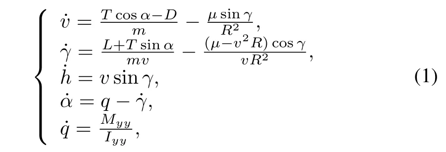
where v,γ,h,αand q represent velocity,flight-path angle, altitude,angle of attack and pitch rate,R=h+REis the altitude of vehicle,REis the radius of the Earth.Iyyis moment of inertia.Left L and draft D are expressed as follows:

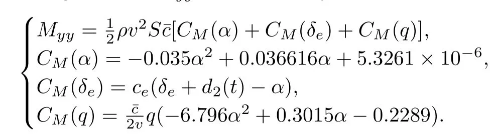
Pitching moment Myyis described by

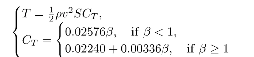
Thrust T is defined as

The system in(1)is linearized with the given cursing condition M a=15,v=15 060 ft/s,h=110 000 ft, γ =0o,q= 0o.The open-loop eigenvalues shown in Fig.1 are−0.895,0.784,−0.00021±0.0362j and 0.00011[26], where−0.895 and 0.784 are the short period oscillation, corresponding to q andα,−0.00021±0.0362j are the phugoid w.r.t.v andγ,0.00011 is the eigenvalue about the altitude modal.It is obvious the nonlinear aircraft in(1)is unstable.

Fig.1.The open-loop eigenvalues of winged-cone model at the given cursing condition.

The engine dynamic ofthe aircraftis expressed by a second order differential equation with the control inputβc

The precise definition of every variable in the equations(1) and(2)is stated in Appendix A.

The composite controlled system contains the equations(1) and(2).The elevator defl ection angleδeand the demand of the engine control inputβcare the control inputs,and the longitudinal velocity v and the altitude h are outputs. Considering the equations(1)and(2),v has the relation with βcandδe,which is derived as

Similarly,the relationship is investigated among h,βcandδe. As

then we have

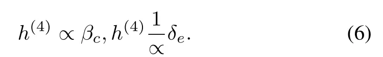
Therefore,βcandδeare explicitly contained in... v and h(4).

The aircraft in(1)and(2)can be included by the general nonlinear formula,

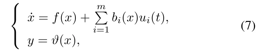
where x∈Rnis the state vector,u(t),ϑ(x)∈Rmare inputs and outputs.f(x)and bi(x)along with the functionϑiare smooth functions on Rn,allowing arbitrary order derivatives to be calculated.

As the system in(7)has m output components,it is considered to produce m subsystems if the input-outputfeedback linearization is executed,where the relative degree of the i-th subsystem is recorded as ri,i=1,···,m.

Assumption 1.Allthe relative degree ri,i=1,···,m of m subsystems are constantand known.The system in(7)does notcontain zero dynamics,which means that the system degree˜r is equal to the sum of relative degrees ri,P

The ri-th derivative of yi=ϑi(x)can be expressed by Lie derivatives

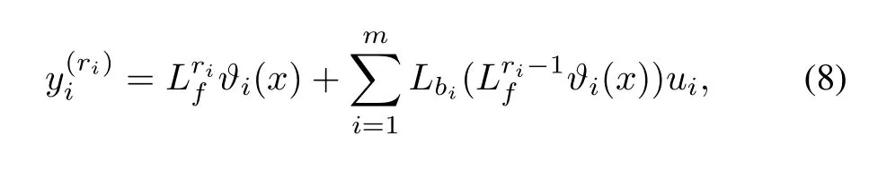
where Lfϑi(x)is the Lie derivative of the functionϑialong the vector field f,

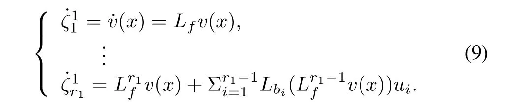
The composite controlled system in(1)and(2)reveals that the system degree is˜r=7.According to(3)and(4),the relative degree of velocity subsystem to inputs is r1=3. The relative degree of altitude subsystem to inputs is r2=4 referring to(6).

It means that the system degree equals to the total relative degrees of subsystems.In other words,the feedback linearization can be executed to reveal that... v and h(4)must be explicitly expressed by the control inputsδeandβc.The original nonlinear model is transformed into two coupling subsystems from inputs to outputs.Therefore we consider the following two subsystems for the cruising control,

Velocity subsystem:

Altitude subsystem:

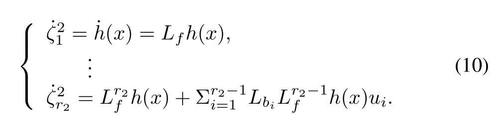
The ri-th derivatives of velocity and altitude dynamics havethe explicit expression with control variables,combining andas follows:

is nonsingular over the entire flightenvelope given in[19−20]. As r1=3 and r2=4,the derivatives of v and h are calculated by the chain rule,

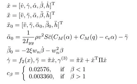
The expressions of˙x,¨x,¨x0,¨α0,¨β0,¨γ,... γ,˜w,Ω,˜πandΠ refer to Appendix A[10].

Remark 1.The feedback linearization transformation aims to explore the explicitcontrolinputs forthe outputs ofvelocity and altitude,which provides the control-oriented subsystems. However,as L3fv(x),L4fh(x)and B(x)are nonlinear,the two subsystems are still nonlinear and coupled.It is easier to design the controller with the explicit control inputs than that with implicit inputs.

According to the formulae of(9)and(10),the generalmodel of subsystems is described as follows,

As external disturbances d1(t)and d2(t)existing in¨βand CM(δe)are considered to be matched,the ri-th subsystem is concluded to the manifold,

Control object:In this paper,the objective is to design a robust continuous sliding mode controller based on velocity and altitude subsystems in the manifold(13),such that the velocity v and the altitude h can track their reference vrand hr,especially existing unknown external disturbances.

III.CONTINUOUS SLIDING MODE CONTROLLER DESIGN WITH DISTURBANCE COMPENSATION FOR AIR-BREATHING HYPERSONIC VEHICLES

In this section,the continuous sliding mode controller is studied for the tracking control.When disturbances exist,the original feedback control law is applied to(11),

where ¯f(x) = [¯f1(x),¯f2(x)]T,¯b(x)= [¯b1(x),¯b2(x)]T, w=[w1,w2]Tis the auxiliary control vector.In this case, the controlled objective(13)is equivalent to the ri-th order integrator system,

where¯di(t)=¯bi(x)∗d(t),i=1,2,j=1,2,···,ri−1.

A.Disturbance Observer Design

The purpose of disturbance observer is to efficiently estimate real-time disturbances.Observed values are used as compensation terms included in control signals.With the compensator,disturbances can be restrained to zero after a finite time,and the controller guarantees the accessibility and the stability before the free-error observation is achieved.

Considering the tracking problem of AHVs,it is presented as ‰

For the differential equation(16),whereσris continuous vector function,the disturbance vector¯d(t)is bounded and has Lipshitz constants L=[L1,L2]T,where|¯d1(t)|≤ L1and|¯d2(t)|≤L2.Therefore,second order observers are used to observe¯d1(t)and¯d2(t)referring to Appendix B,which are expressed in the form of vectors as follows:

whereλ0,λ1,λ2are gains of the o bserver,converges to d¯(t)in finite time.

Remark 2.The convergence proof of disturbance observer can refer to literatures[27−28].In addition,the l-th order observer provides more accurate derivatives than the p order observer,p≤l[29].By(17),z1can converge to¯d(t)in finite time,which guarantees thatobservation errors converge to zero in finite time.

B.Continuous Sliding Mode Controller Design

For the subsystem expressed in (15),define σ = [σ1,σ2,···,σri]T,the sliding surface is as follows:

where¯C=[0,cri−1ri−1λri−1,···,c1

ri−1λ].If the derivative is designed as

where edi(t)= ¯di(t)−zi1(t),ℓ1＞ 0,ℓ2＞ 0,0＜ o1＜ 1, o2＞1,sigoi(sri)=|sri|oisgn(sri).We can getthe following theorem.

Theorem 1.For system(15),if the continuous controller is used

the reachability of srihas two cases:

1)if the observer error edi(t)=0,system states reach the sliding manifold sri=0 in finite time;

2)ifthe observererror edi(t)/=0,system states reach theψ neighborhood of sri=0 in fi nite time and never escape from the region,where

Proof.The Lyapunov function is selected aswhereis positive definite.

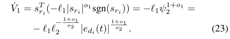
Case 1:edi(t)=0,the time derivative of V1

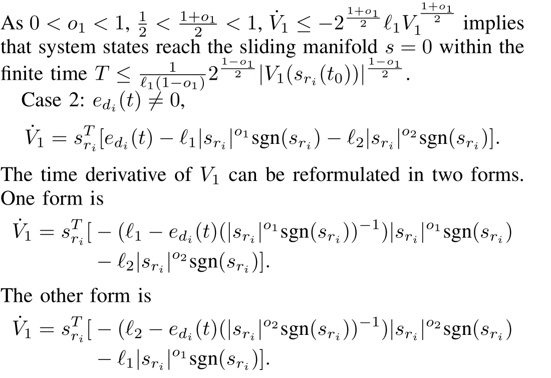
The other case is|sri|=ψ2,

From the two cases,it can be concluded thatthe system states can reach the surface|sri|=ψin finite time.

The region|sri|≤ ψ =min{ψ1,ψ2}is an attractive area for the states of system(15).System states do not escape from the region once reach it.To prove that,we need only to show that any system state on the boundary |sri|= ψ = min{ψ1,ψ2},never enters the region of |sri|＞ ψ =min{ψ1,ψ2}again.According to the above analysis,the time derivative of V1(sri)on the boundary |sri|=min{ψ1,ψ2}is always negative definite refereing to (22)and(23),namely˙V1(sri)=−ℓ,ℓ＞0.This means|sri| is monotonically decreasing,system states on the boundary enter the region|sri|＜ψand never escape it.

In sum,with the controller(21),the states of system(15) always reach the sliding mode surface sri=0 in finite time without observation errors and arrive at the region|sri|≤ψ in finite time if observation errors exist. □

C.Continuous Sliding Mode Controller with Disturbance Compensation for The Tracking Control of AHVs

Define the tracking error as ev(t)=v(t)−vr(t)and eh(t)=h(t)−hr(t),such that

For disturbances¯d1(t)and¯d2(t),the disturbance observer is used to estimate them.We have the corollary forobservation errors.

Corollary 1.The disturbance observation errors,edi(t)= ¯di(t)−zi1(t),i=1,2,are obviously bounded and should converge to zero after a finite time T,which is

whereτi,i=1,2 is bounded constants.

Theorem 2.For system(24)and(25),if the following continuous sliding mode controllerwith disturbance compensation is used,

the velocity v and the altitude h are guaranteed to asymptotically track reference signals vrand hrwith switching modes svand sh,where z11(t)and z21(t)are compensation terms for disturbances¯d1(t)and¯d2(t),respectively,obtained by(17).

Proof.Via feedback linearization,two decoupled subsystems are presented.The velocity switching mode is designed in the manifold,

whereλv= [c22λ2,c12λ,1],Ev= [ev,˙ev,¨ev]T.The time derivative of svis

where¯λv=[0,c22λ2,c12λ].

The altitude switching mode is considered as

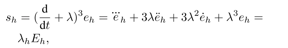
where¯λh=[0,c33λ3,c23λ2,c13λ].

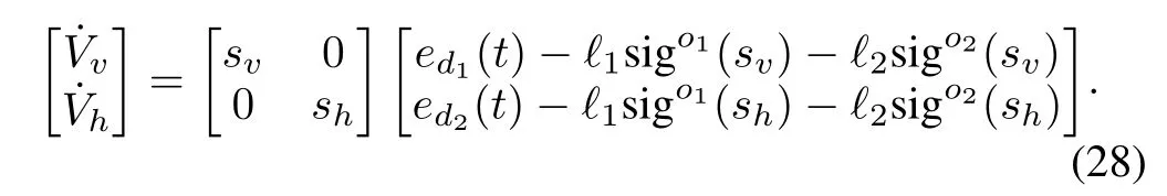
Combining the equations of˙svand˙sh,we have the compact expression

The control variables in the above formula are replaced by the designed control law(27),then the derivative of V is

Corollary 1 shows the property of observation errors edi(t), which is bounded and converges to zero after a finite time. According to Theorem 2,when edi(t)/=0,system states would reach neighborhoods of switching modes with respect to edi(t).When ed1(t)/=0,system states[ev,˙ev,¨ev]reachtheψvregion of sv=0,ψvWhen ed2(t)/=0,system statesregion of sh=0,ψh=mineventually stabilizes to zero after a finite time,system states also reach sv=0 and sh=0 in fi nite time.

When sv=0 and sh=0,the dynamics of tracking error system on sliding modes sv=0 and sh=0 are obtained,

It can be concluded that ev=c1e−λt,eh=c2e−λt,where c1,c2are undetermined constants,e is the natural exponent. Therefore,evand ehcan asymptotically converge to zero,v and h can track reference signals vrand hr,respectively.□

Remark 3.The figure of the function|sri|oisgn(sri)is presented in Fig.2.It is obvious that the function is continuous.Therefore,the control law in(27)is also continuous. For the continuous controller,the chattering is eliminated. Note thatsystem states arrive ata smallneighborhood of sri, i=1,2 before observation errors edi(t)reach zero,which is considered to be the cost of eliminating the chattering. The boundary layer method keeps the width of convergence region no matter what edi(t)is,and the convergence is asymptoticalto the smallregion.The proposed method enables the asymptoticalconvergence to zero when edi(t)reaches zero and avoids chattering.

Remark 4.The terms−ℓ1sigo1(sri)−ℓ2sigo2(sri)in the controllaw(27)can increase the convergence rate.When system states are far away from sri=0,the term−ℓ2sigo2(sri) would accelerate the convergence.When system states are very close to sri=0,the term−ℓ1sigo1(sri)help the convergence. Refer to Fig.2,|sri|oisgn(sri)with oi=0.5,oi=1.5 and oi=2.2.

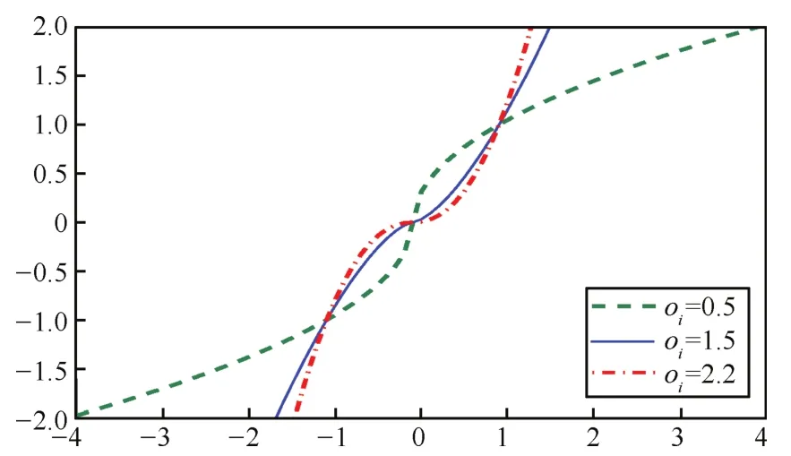
Fig.2. The continuous function|sri|oisgn(sri)with different oivalues.

IV.SIMULATION

In this section,simulation is executed to demonstrate the effectiveness of the proposed method.

As a representative case study,the hypersonic vehicle is assumed to trim at v=15 060 ft/s and h=110 000 ft,and the aerodynamic coefficients and model parameters are given in Table I.

Parameters of the sliding mode controller areλv=λh=1,ℓ1= ℓ2=10,o1=0.6 and o2=1.5.Parameters of disturbance observer are designed asλ0=3,λ1=1.5, λ2=1.1,L1=15,L2=50.

A.Tracking Control

The reference velocity is 14 960 ft/s and the reference altitude is 110 200 ft.During the tracking process,the vehicle is perturbed by

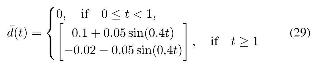
The continuous sliding mode controller is adopted,where the finite time disturbance observer is used as the compensator to reject disturbance.Figs.3(a)and 3(b)show that the designed observer can work effectively to exactly estimate disturbances in fi nite time,where dotted lines represent actual disturbances and solid lines depict observed values. The observed values z11and z21have well approximation to disturbances¯d1and¯d2after a finite time.

TABLE I AERODYNAMIC AND INERTIAL COEFFICIENTS

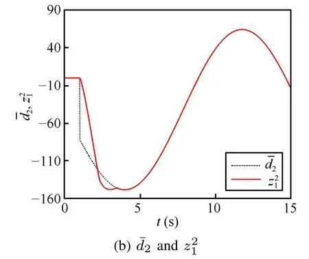
Fig.3. Real disturbance values and estimated values.

Fig.4. The positive boundaries of velocity and altitude switching modes.

As stated in Theorem 1,before estimated errors become zero,the velocity switching mode and the altitude switching mode arrive at small regions with respect to estimated errors. In other words,if the track error of velocity ed1(t)/=0, evreaches theψvregion of sv= 0,whereψv=For the same reason,if the tracking error ed2(t)/=0 of altitude,ehalso runs into theψhregion of sh=0,whereψhOnce tracking errors edi(t)stabilizes to zero aftera finite time, system states also reach sv=0 and sh=0 in finite time.Fig.4 presents the boundaries ofthe two smallregions,whereψvand ψhwith solid lines describe positive boundaries for velocity and altitude switching modes,and

Fig.5 further describes curves of svand sh,which locate in small regions before tracking errors reach zero,restrained

Fig.6 provides the continuous control lawsβcandδeto avoid the chattering.Simultaneously,tracking results of velocity and altitude are also displayed in Fig.6,where velocity and altitude are both asymptotically stabilize attheir reference commands.It exhibits good robustness against disturbances with the composite controller.The boundary layer method is executed to compare with the proposed method.The sign function is replaced by the saturation function and the finite time disturbance observeris stillused as the compensator.The width of the saturation function isτ=0.5,the gain l1=20. The simulation results are illustrated in Fig.6 with dashed lines.The chattering has been eliminated,but the system responses are stillslower than thatwith the proposed method.

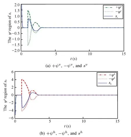
Fig.5. Switching mode variables located in their regions.

B.Robustness

It can be observed that the composite control has finished the tracking of velocity and altitude within ten seconds in the previous simulation.The hypersonic aircraft is expected to track step commands,where vr=14 960 ft/s and hr= 110 200 ft change to vr=14 870 ft/s and hr=110 360 ft at t=20 s.The disturbances also change at t=35 s,which are designed as follows:

The robustness ofcontrolleris checked here.Allparameters are set the same as the previous simulation.The varying disturbances are effectively estimated by the finite time observer,shown in Fig.7,where dotted lines represent disturbances, solid lines are provided by estimated values.

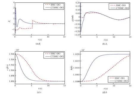
Fig.6.Control laws and output responses,continuous TSMC with DO,saturation SMC with DO.

Fig.7. Estimated values for¯d1and¯d2.

Fig.8 presents new boundaries of svand shconsidering new varying disturbances.Switching mode variables svand share firstly restrained to small regions,and then the two switching mode variables arrive atzero when estimated errors converge to zero.

The continuous control laws illustrated in Fig.9.v and h keep convergentto reference signals,where the robustness of the continuous controller is illustrated.Velocity and altitude are not perturbed even if new disturbances are added at t=35 s,and stillkeep welltracking to step reference signals.

Fig.8.Switching modes and their regions.

Fig.9.Control laws and output responses.

V.CONCLUSION

In this paper,a composite continuous controlleris discussed for the tracking problem of hypersonic vehicles.The system model is linearized to velocity and altitude subsystems. The continuous controller is designed to reduce chattering. The finite time disturbance observer is introduced to reject disturbances.Because the discontinuous term is replaced by continuous terms,switching modes of velocity and altitude arrive at small regions which vary depending on disturbance observation errors.When observation errors disappear,the observer converges to disturbance signals in finite time.It turns out that restrained regions to switching modes become zero and tracking errors of velocity and altitude asymptotically converge to zero.The method has significantly improved boundary layer method.Simulations have proved the effectiveness of the proposed continuous sliding mode controlwith disturbance observer for the tracking control of AHVs and high convergence rate is also provided.

APPENDIX A

Nomenclature:

v−speed of sound

γ−flight-path angle

h−altitude

α−angle of attack

q−pitch rate

T−thrust

D−drag

L−lift

CT(β)−thrust coefficient

CD(α)−drag coefficient

CL(α)−lift coefficient

CM(q)−pitch rate contribution to moment

CM(α)−angle of attack contribution to moment

CM(δe)−elevator deflection contribution to moment

m−mass

RE−radius of the Earth

R−radial distance from Earth's center

¯c−mean aerodynamic chord

cβ−throttle coefficient in CT

ce−elevator coefficient in CM(δe)

Iyy−moment of inertia

Myy−pitching moment

S−reference area

δE−elevator angular deflection

β−throttle setting

βc−control contribution to throttle settingβ

wn−natural frequency for throttle settingβ

ξ−damping ratio for throttle settingβ

µ−gravitational constant

ρ−density of air

Expression:

APPENDIX B

Considering the system ˙x(t)=y(t)+g(t),allderivatives˙g(t), ¨g(t),···,g(p−1)(t)of the disturbance term g(t)are assumed to be bounded,such that there is a known Lipshitz constant L＞0 for g(p−1)(t).

For a continuous function x(t)defined t≥ 0,if y(t)is Lebesgue-measurable,when input noises of x(t)and y(t)are zero,the exact finite time observer for g(t)can be established as follows:with enough large parametersλi,i=0,···,p,z0,z1,···,zpcan converge to x,g(t),···,g(p−1)(t)in fi nite time.

REFERENCES

[1]Fidan B,Mirmirani M,Ioannou P A.Flight dynamics and control of air-breathing hypersonic vehicles:review and new directions.In:Proceedings of the 2003 AIAA International Space Planes and Hypersonic Systems and Technologies.Norfolk,USA:AIAA,2003.

[2]Fiorentini L,Serrani A,Bolender M A,Doman D B.Nonlinear robust adaptive control of flexible air-breathing hypersonic vehicles.Journal of Guidance,Control,and Dynamics,2009,32(2):401−416

[3]Sigthorsson D O,Jankovsky P,Serrani A,Yurkovich S,Bolender M, Doman D B.Robust linear output feedback control of an air-breathing hypersonic vehicle.Journal of Guidance,Control,and Dynamics,2008, 31(4):1052−1065

[4]Zhu Y J,Shi Z K.Several problems of flight characteristics and flight control for hypersonic vehicles.Flight Dynamics,2005,23(3):5−8

[5]Gregory I M,McMinn J D,Chowdhry R S,Shaughnessy J D.Hypersonic Vehicle Model and Control Law Development Using H∞and µSynthesis,NASA Technical Memorandum,USA,NASA TM-4562, 1994.

[6]Lind R.Linear parameter-varying modeling and controlof structuraldynamics with aero-thermodynamic effects.Journal of Guidance,Control, and Dynamics,2002,25(4):733−739

[7]Oppenheimer M W,Doman D B.Control of an unstable,nonminimum phase hypersonic vehicle model.In:Proceedings of the 2006 Aerospace Conference.Big Sky,MT:IEEE,2006.1−22

[8]Gibson T E,Annaswamy A M.Adaptive controlof hypersonic vehicles in the presence of thrust and actuator uncertainties.In:Proceedings of the 2008 AIAA Guidance,Navigation and Control Conference and Exhibit.Hawali,USA:AIAA,2008.

[9]Serrani A,Zinnecker A M,Fiorentini L,Bolender M A,Doman D B.Integrated adaptive guidance and control of constrained nonlinear air-breathing hypersonic vehicle models.In:Proceedings of the 2009 American ControlConference.St.Louis,USA:IEEE,2009.3172−3177

[10]Wang Q,Stengel R F.Robustnonlinear controlof a hypersonic aircraft. Journal of Guidance,Control,and Dynamics,2000,23(4):577−585

[11]Xu J H,Mirmirani M,loannou P A.Adaptive sliding mode control design for a hypersonic flightvehicle.Journal of Guidance,Control,and Dynamics,2004,27(5):829−838

[12]Bowcutt K G.Multidisciplinary optimization of airbreathing hypersonic vehicles.Journal of Propulsion and Power,2001,17(6):1184−1190

[13]Jiang C H,Zhang C Y,Zhu L.Research of robust adaptive trajectory linearization control based on T-S fuzzy system.Journal of Systems Engineering and Electronics,2008,19(3):537−545

[14]Zhu L,Jiang C S,Zhang C Y.Adaptive trajectory linearization control for aerospace vehicle based on RBFNN disturbance observer.Acta Aeronautica etAstronauticaSinica,2007,28(3):673−677

[15]Hu X X,Wu L G,Hu C H,Gao H J.Adaptive sliding mode tracking control for a flexible air-breathing hypersonic vehicle.Journal of the FranklinInstitute,2012,349(2):559−577

[16]Yu S H,Yu XH,Shirinzadeh B,Man Z H.Continuous finite-time control for robotic manipulators with terminalsliding mode.Automatica,2005, 41(11):1957−1964

[17]Slotine J J,Sastry S S.Tracking control of non-linear systems using sliding surfaces with application to robot manipulators.International Journal of Control,1983,38(2):465−492

[18]Slotine J J,Li W P.Applied Nonlinear Control.New Jersey:Prentice Hall,1991.

[19]Li S H,Sun H B,Sun C Y.Composite controldesign for an air-breathing hypersonic vehicle.Proceedings of the Institution of Mechanical Engineers,Part I:Journal of Systems and Control Engineering,2012,226(5): 651−664

[20]Sun H B,Li S H,Sun C Y.Finite time integralsliding mode controlof hypersonic vehicles.Nonlinear Dynamics,2013,73(1−2):229−244

[21]Zong Q,JiY H,Zeng F L,Liu H L.Outputfeedback back-stepping control for a generic hypersonic vehicle via small-gain theorem.Aerospace Science and Technology,2012,23(1):409−417

[22]Zong,Q,Wang J,Tao Y.Adaptive high-order dynamic sliding mode control for a flexible air-breathing hypersonic vehicle.International Journal of RobustNonlinear Control,2013,23(15):1718−1736

[23]Sigthorsson D O,Jankovsky P,Serrani A,Yurkovich S,Bolender M, Doman D B.Robust linear output feedback control of an air-breathing hypersonic vehicle.Journal of Guidance,Control and Dynamics,2008, 31(4):1052−1066

[24]Bolender M A,Doman D B.Nonlinear longitudinaldynamicalmodelof an air-breathing hypersonic vehicle.Journal of Spacecraft and Rockets, 2007,44(2):374−387

[25]Shaughnessy J D,Pinckney S Z.Hypersonic Vehicle Simulation Model: Winged-Cone Configuration,NASA Technical Memorandum,USA, NASA TM-102610,1991.

[26]Li F H.Guidance and Control Technology of Hypersonic Aircrafts. Beijing:China Astronautic Publishing House,2012.

[27]Levant A.High-order sliding modes,differentiation and outputfeedback control.International Journal of Control,2002,76(9−10):924−9412

[28]Shtessel Y B,Shkolnikov A,Levant A.Smooth second-order sliding modes:missile guidance application.Automatica,2007,43(8): 1470−1476

[29]Levant A.Robust exact differentiation via sliding mode technique. Automatica,1998,34(3):379−384

Qun Zong Received the bachelor,master,and Ph.D. degrees all in automatic control from Tianjin University,in 1983,1995 and 2002,respectively.Since 1983,he has been with the School of Electrical Engineering and Automation,Tianjin University,where he is currently a professor.His research interests include complex system modeling and flightcontrol. Corresponding author of this paper.

Bailing Tian Received his Ph.D.degree in automatic controlfrom Tianjin University in 2011.Since 2011,he has been with the Schoolof Electrical Engineering and Automation,Tianjin University,where he is currently a lecturer.His research interests include trajectory optimization,guidance and control.

Wei Xu Received the Ph.D.degree in electrical engineering from the Institute of Electrical Engineering,Chinese Academy of Sciences in 2008.He is currently a professor with the School of Electrical and Electronic Engineering,Huazhong University of Science and Technology.His research interests include controland electromagnetic design for electric machines.

Received her Ph.D.degree in control theory and control engineering from School of Automation,Southeast University,in 2012.Since 2012,she is a lecturer at the School of Electricaland Automation Engineering,Tianjin University. Her research interests include sliding mode control, nonlinear system control,and intelligent control.

Manuscriptreceived October 15,2013;accepted April11,2014.This work was supported by National Natural Science Foundation of China(61125306, 61273092,61301035,61304018,and 61411130160),National High-Technology Research and Development Program of China(2014AA051901), Tianjin Science and Technology Supporting Program(14JCQNJC05400), Research Innovation Program of Tianjin University(2013XQ0101),Hubei Science and Technology Supporting Program(XYJ2014000314),Aeronautical Science Foundation of China Supported by Science and Technology on Aircraft Control Laboratory(20125848004),and China Post-doctoral Science Foundation(2014M561559).Recommended by Associate Editor Bin Xian

:Chaoxu Mu,Qun Zong,Bailing Tian,WeiXu.Continuous sliding mode controllerwith disturbance observerforhypersonic vehicles.IEEE/CAA Journalof Automatica Sinica,2015,2(1):45−55

Chaoxu Mu,Qun Zong,and Bailing Tian are with the Departmentof Electrical Engineering and Automation,Tianjin University,Tianjin 300072,China (e-mail:cxmu@tju.edu.cn;zongqun@tju.edu.cn;bailing−tian@tju.edu.cn).

Wei Xu is with the School of Electrical and Electronic Engineering, Huazhong University of Science and Technology,Wuhan 430074,China(email:weixu@hust.edu.cn).