Local Regularity for a 1D Compressible Viscous Micropolar Fluid Model with Non-homogeneous Temperature Boundary

SUN Lin-lin,LIANG Tie-wang,ZHANG Jian-peng

(1.College of Science,Donghua University,Shanghai 201620,China;2.Department of Infomation and Arts Design,Henan Forestry Vocational College,Luoyang 471002,China)

Local Regularity for a 1D Compressible Viscous Micropolar Fluid Model with Non-homogeneous Temperature Boundary

SUN Lin-lin1,LIANG Tie-wang2,ZHANG Jian-peng1

(1.College of Science,Donghua University,Shanghai 201620,China;2.Department of Infomation and Arts Design,Henan Forestry Vocational College,Luoyang 471002,China)

In this paper,we discuss the local existence of Hi(i=2,4)solutions for a 1D compressible viscous micropolar fluid model with non-homogeneous temperature boundary. The proof is based on the local existence of solutions in[1].

compressible Navier-Stokes equations;micropolar fl uid;the initial boundary value problem;non-homogeneous temperature boundary

§1. Introduction

The present paper is concerned with the local existence of Hi(i=2,4)solutions to the system of one-dimensionalcompressible viscous micropolar fluid modelwith non-homogeneous temperature boundary.This system is a kind of viscous compressible Navier-Stokes equations describing the motion of a heat-conducting micropolar fluid,which belongs to a class of fluids with nonsymmetric stress tensor called polar fluids.Precisely in the Lagrangian coordinate, such a system can be written as follows

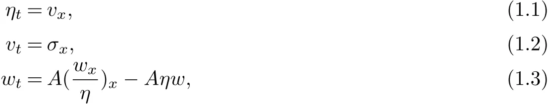
where for(x,t)∈[0,1]×[0,T](T＞0)is the Lagrangian mass coordinate and

denote stress,heat flux,pressure and internal energy,respectively and A＞0 is a constant.In addition,

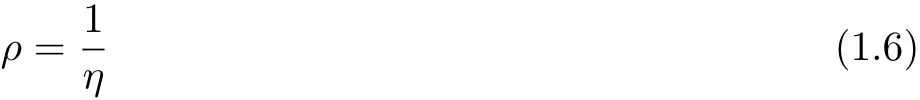
denotes the density of the fluid.Meanwhile,we consider(1.1)～(1.5)subject to the following initial conditions

and the following boundary conditions

whereη0(x),v0(x),w0(x),θ0(x)are given functions.We also assume as in Nermina Mujakovic’s article

where m＞0 is a constant.

The research of1Dcompressible Navier-Stokes system has obtained a great ofresults.Specifically,the crucialpoint to the research is that in 1D case under the Lagrangian coordinate,the specific volumeηcan be represented by other unknown variables,and the positive upper and lower bounds can be derived in the respective initialboundary problems.[2-4]have studied the Cauchy problem.As the domain is unbounded and the Poincar´e inequality is not available,the authors discussed it in small initial data condition.There are also a lot of works concerning the initial boundary problems(see,e.g.,[5-24]).They have obtained many results concerning the global existence,regularity and asymptotic behavior.Qin[2223]also obtained a series of properties about the exponential stability and attractors of the system.Recently,Mujakovi´c has studied the non-homogeneous boundary value problems,such as velocity boundary v,momentum w and temperatureθare non-homogeneous(see,e.g.,[1,25]).Actually,this paper is based on the local existence results in Mujakovi´c[1]and improves his result.

In this paper,constants Ci(i=1,2,3,4)denote the universal constants depending on the Hi[0,1](i=1,2,3,4)spatial norms of(η0(x),v0(x),w0(x),θ0(x))and Wi,∞[0,T](i= 1,2,3,4)spatialnorms of(u0(t),u1(t)).

Now,we state our main results in this paper

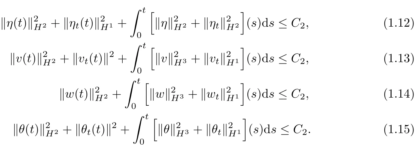
Theorem 1 If(1.10)～(1.11)are satisfied,(η0(x),v0(x),w0(x),θ0(x))∈H2[0,1]and (u0(t),u1(t))∈W2,∞[0,T],then there exists a time 0≤T0≤T,such that problem(1.1)～(1.9) admits a H2-local solution(η(t,x),v(t,x),w(t,x),θ(t,x))∈L∞([0,T0),H2[0,1])and the following estimates hold for any t∈[0,T0),

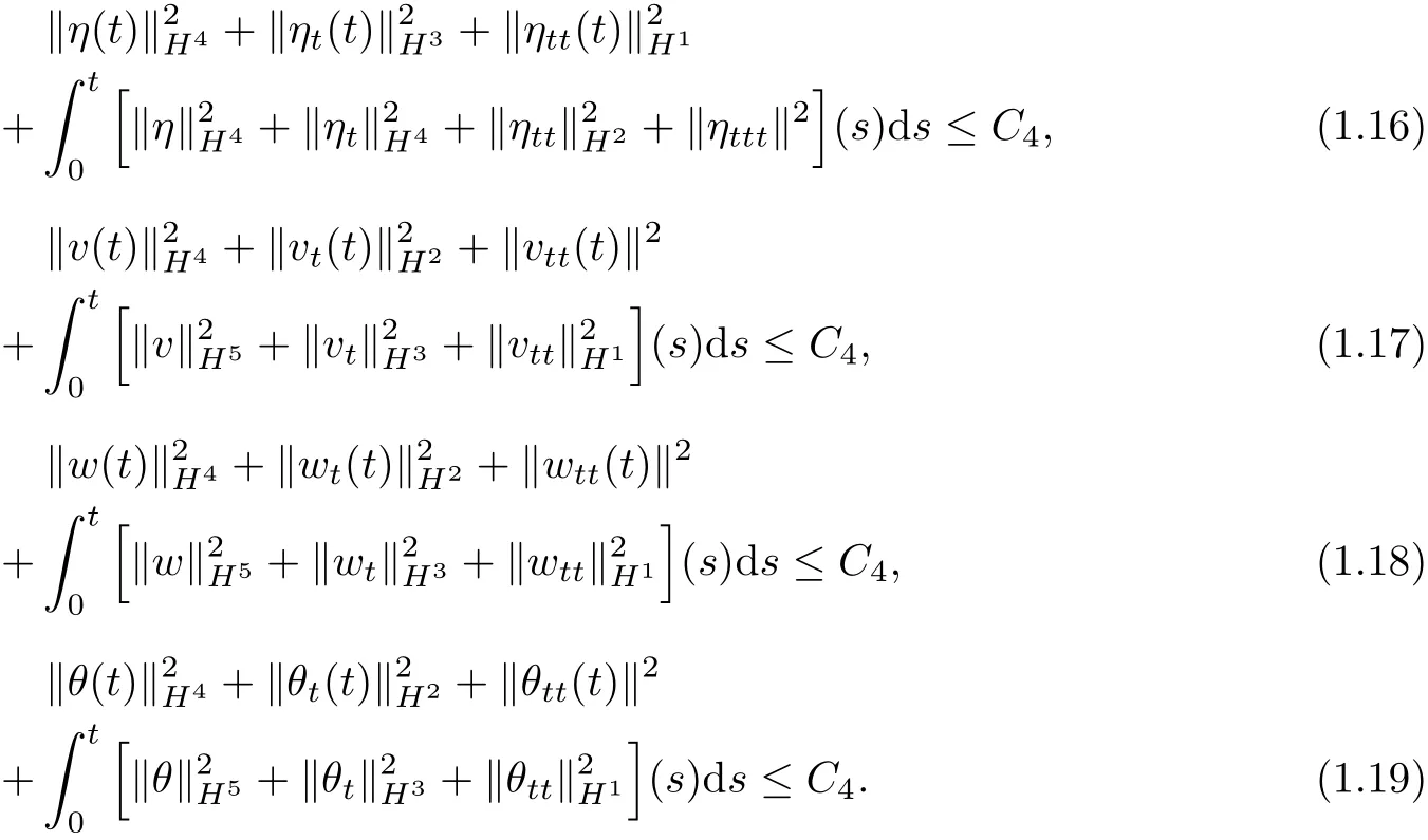
Theorem 2 If(1.10)～(1.11)are satisfied,(η0(x),v0(x),w0(x),θ0(x))∈H4[0,1]and (u0(t),u1(t))∈W3,∞[0,T],then there exists a time 0≤T0≤T,such that problem(1.1)～(1.9) admits a H4-local solution(η(t,x),v(t,x),w(t,x),θ(t,x))∈L∞([0,T0),H4[0,1])and the following estimates hold for any t∈[0,T0],

We organize the paper as follows:Section 2 is asserted for the proof of Theorem 1 and Section 3 is arranged as for the proof of Theorems 2.

§2. Local Existence in H2

Lemma 2.1 Under the assumptions of Theorem 1.1,there exists a time 0≤T0≤T, such that for all t∈[0,T0),there holds

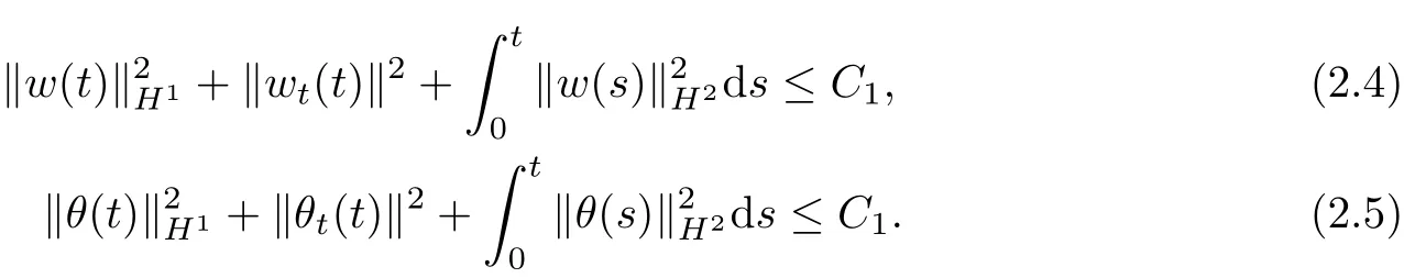
Proof We can easily get(2.1)～(2.5)from Theorem 2.1 and Lemma 5.2 in[1].

Lemma 2.2 The following estimate holds for all t∈[0,T0),

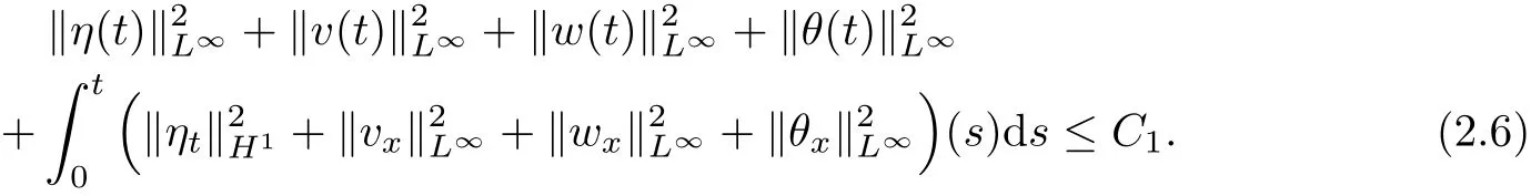
Proof By Lemma 2.1 and the following inequalities

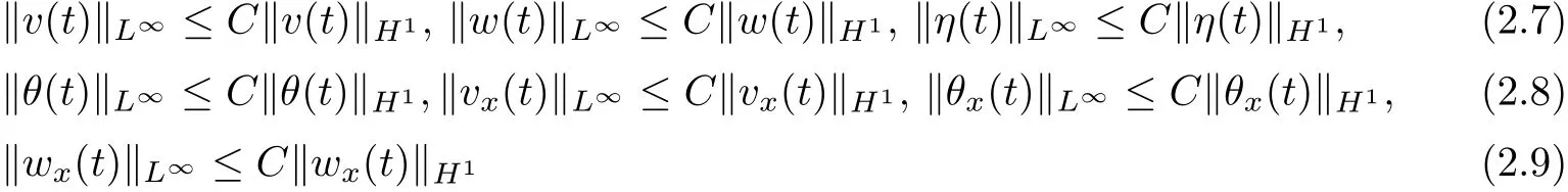
and also from(1.1),

we can get estimate(2.6).The proof is complete.

Lemma 2.3 For all t∈[0,T0),there holds

Proof Differentiating(1.2)with respect t,multiplying the resulting equation by vt,using Lemma 2.1,we deduce that

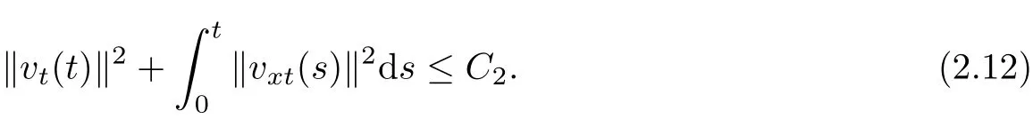
Also from(1.2),using Lemma 2.1,the interpolation inequality and Young’s inequality,we have for anyε＞0,

which gives forε＞0 smallenough,

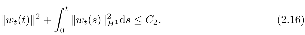
Similarly,we derive from(1.3)forε＞0 smallenough,

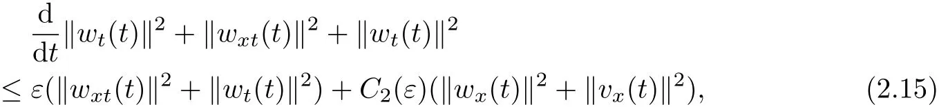
which gives

Meanwhile,we can deduce from(1.3)forε＞0 smallenough,

which gives

Similarly,we derive from(1.4)forε＞0 small enough,

which gives

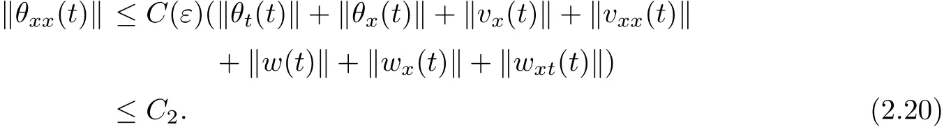
From(1.4),we can obtain,

which gives for anyε＞0,

From Lemma 2.1 and(2.12),(2.15),we arrive

As we know

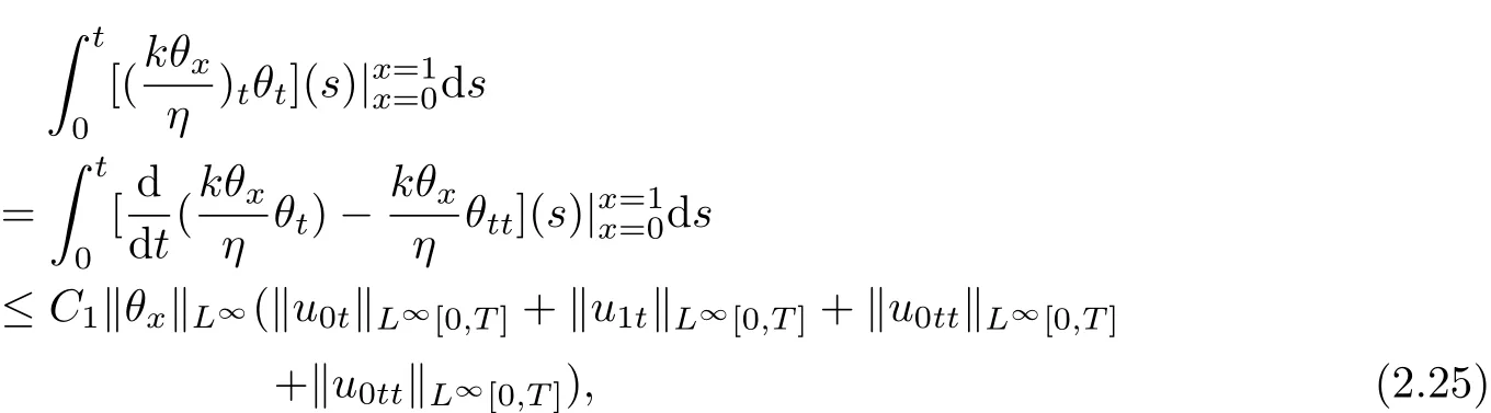
as(u0(t),u1(t))∈W2,∞[0,T]and‖θx‖L∞≤C1(‖θx‖1/2‖θxx‖1/2+‖θx‖),then we know that

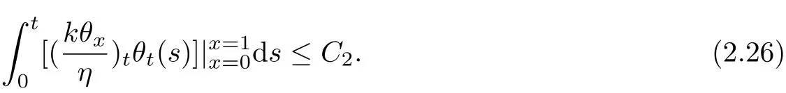
Thus the estimate(2.11)follow from(2.12),(2.14),(2.15),(2.17),(2.19),(2.23)and(2.26). The proof is complete.

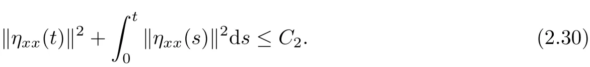
Lemma 2.4 For all t∈[0,T0),there holds

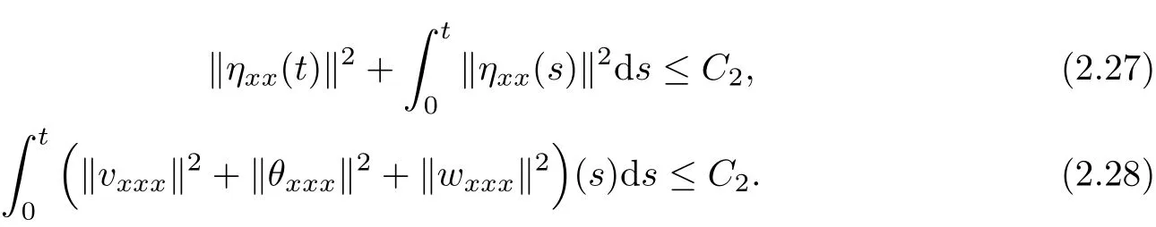
Proof Diff erentiating(1.2)with respect to x,multiplying the resulting equation byηxx/η and using(1.1)(ηtxx=vxxx),we can see that for anyε＞0

which,combined with Lemma 2.1～Lemma 2.3,gives

Differentiating(1.2)～(1.4)with respect to x respectively,using Lamma 2.1～Lemma 2.3,we can see that

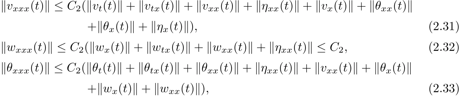
which gives(2.28).The proof is complete.

Proof of Theorem 1 By Lemma 2.1～Lemma 2.4,we have proved the local existence of H2-solution of problem(1.1)～(1.9).

§3. Local Existence in H4

Lemma 3.1 Under the assumptions of Theorem 2,then for all t∈[0,T0),where T0is defined in Lemma 2.1,there holds

whereεis a suffi ciently smallpositive constant.

Proof We easily infer from(1.2)and Lemma 2.1～Lemma 2.4 that

Diff erentiating(1.2)with respect to x and utilizing Lemma 2.1～Lemma 2.4,we have

or

Diff erentiating(1.2)with respect to x twice,using Lemma 2.1～Lemma 2.4 and the interpolation inequalities,we have

or

In the same manner,we deduce from(1.3)and(1.4)that

or

and

or

Diff erentiating(1.2)with respect to t and utilizing Lemma 2.1～Lemma 2.4,we deduce that

which,together with(3.7),(3.9)and(3.14),implies

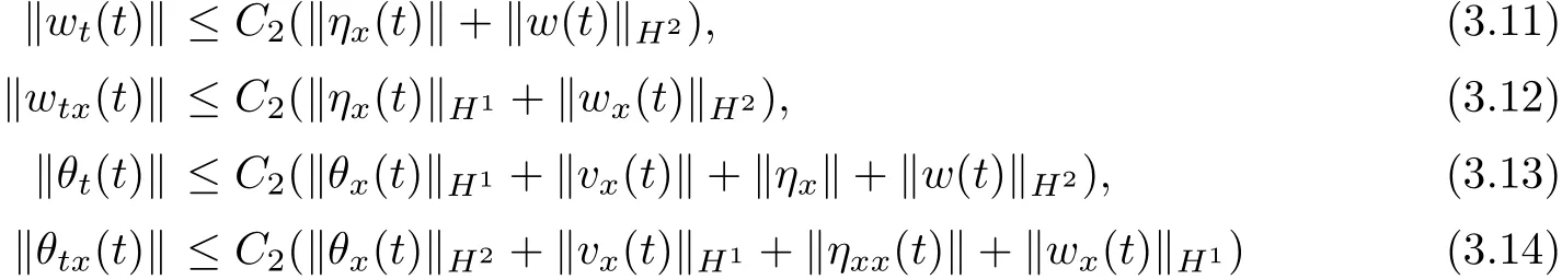
Analogously,we derive from(1.3)～(1.4)and Lemma 2.1～Lemma 2.4 that

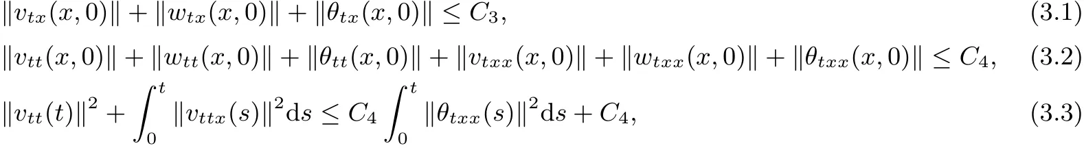
which,combined with(3.11)～(3.14),(3.17)～(3.18)and(3.7),give

Hence we obtain(3.1)～(3.2).

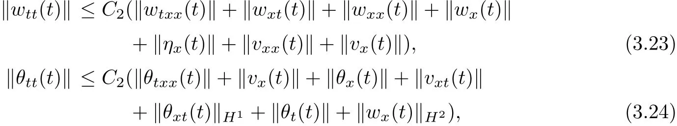
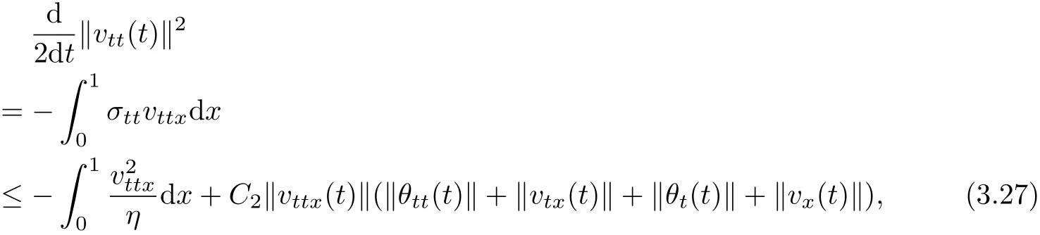
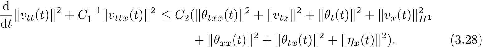
Now diff erentiating(1.2)with respect to t twice,multiplying the resulting equation by vttin L2(Ω)and using(1.1)and Lemma 2.1～Lemma 2.4,we deduce

which,along with(3.24),implies

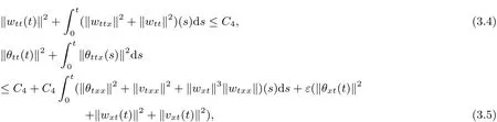
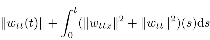
Thus estimate(3.3)follows from Lemma 2.1～Lemma 2.4,(3.2)and(3.28). Analogously,we obtain from(1.3)that

which,integrated over(0,t),t∈[0,T0),implies

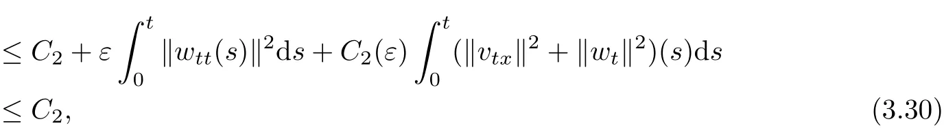
Hence(3.4)follows.

In the same way,we can obtain from(1.4)

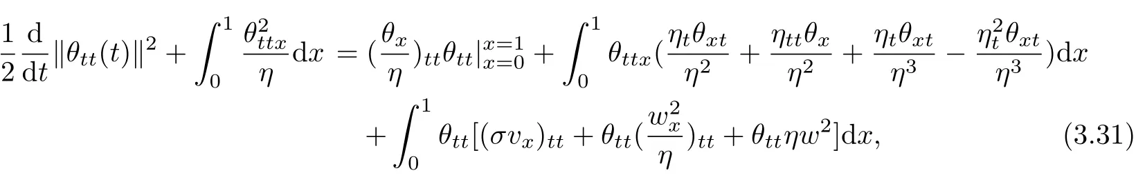
which implies

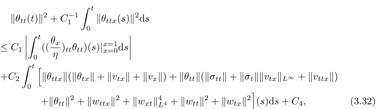
i.e.,

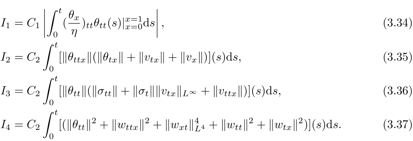
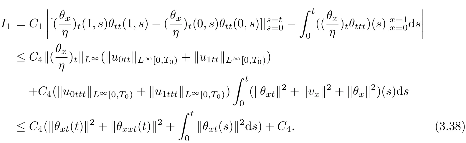
where

As we know

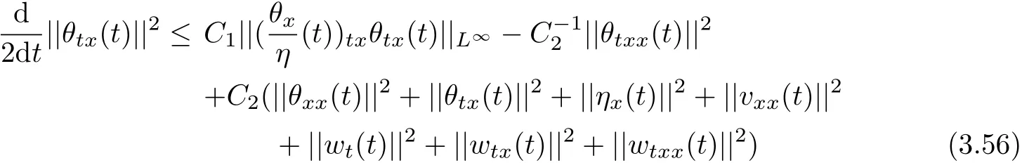
For estimating‖θxxt(t)‖2,we diff erentiate(1.4)with t and use Lemma 2.1～Lemma 2.4,to obtain that for anyε＞0,

So we get

We also easily know that for anyε＞0,

By Lemma 2.1～Lemma 2.4,and the interpolation inequalities,we derive

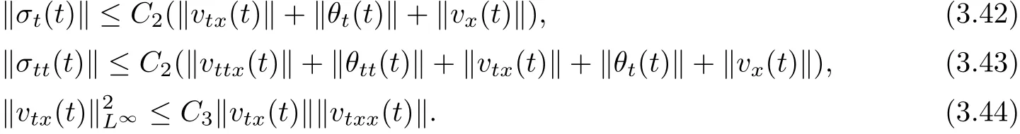
We can get

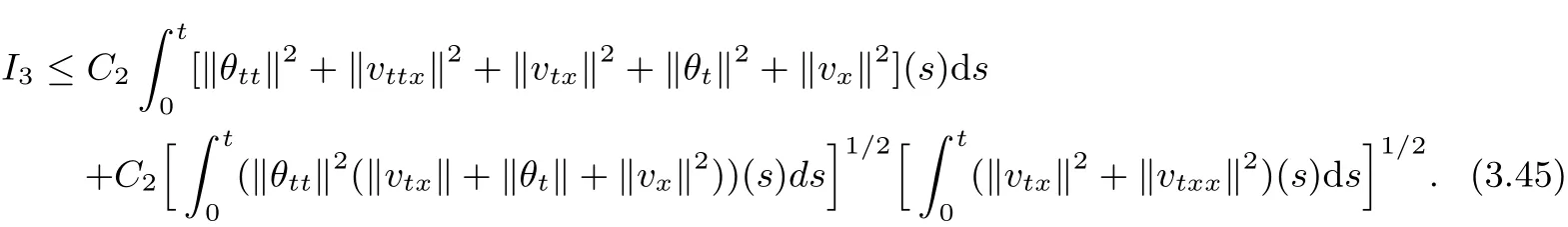
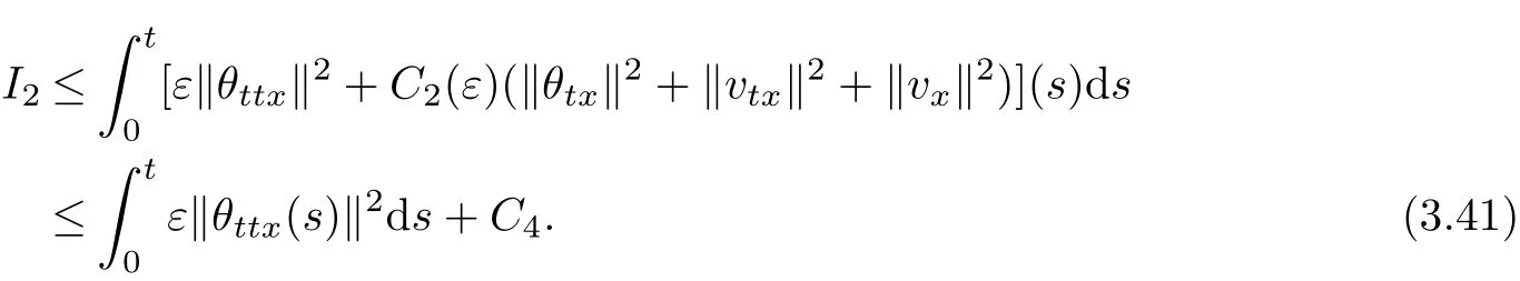
Thus from(3.42)～(3.44)and Lemma 2.1～Lemma 2.4,it follows for anyε＞0,

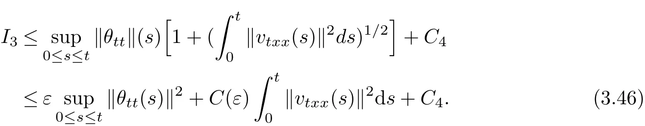
As the interpolation inequality,we know that

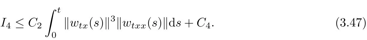
By(3.40)～(3.41),(3.46)～(3.47)and taking the supremum on the right-hand side of(3.43), we can obtain(3.5).The proof is complete.

Lemma 3.2 For all t∈[0,T0),there holds for anyε＞0,

Proof See,e.g.,Lemma 2.5,[22]and(3.48)can be obtained immediately.

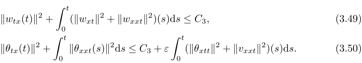
Differentiating(1.3)with respect to x and t,multiplying the resulting equation by wtxin L2(Ω)and integrating by parts,we infer from(1.3)

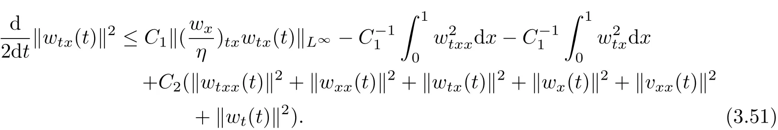
Differentiating(1.3)with respect to t and both to x and t respectively,we can see

Hence it follows from(3.52)～(3.53)

which leads to(3.49).

Analogously,we also deduce from(1.4)and(3.52)

and differentiating(1.4)with respect to t and x,we can see

which,combined with Lemma 2.1～Lemma 2.4,(3.49)and the Young’s inequality,implies estimate(3.50).The proof is now complete.

Lemma 3.3 For all t∈[0,T0),there holds

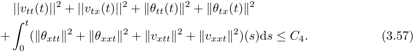
Proof Adding up(3.3),(3.5),(3.48)and(3.50)and takingεsuffi ciently small,also utilizing the fact based on(3.48)

we can immediately obtain(3.57).The proof ends here.

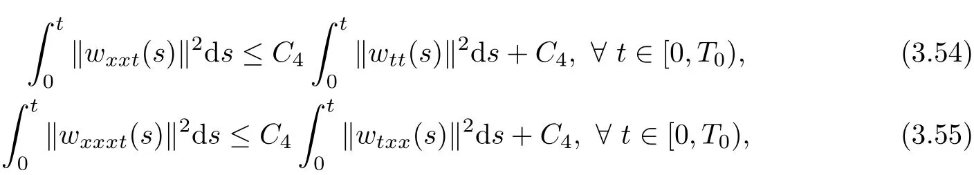
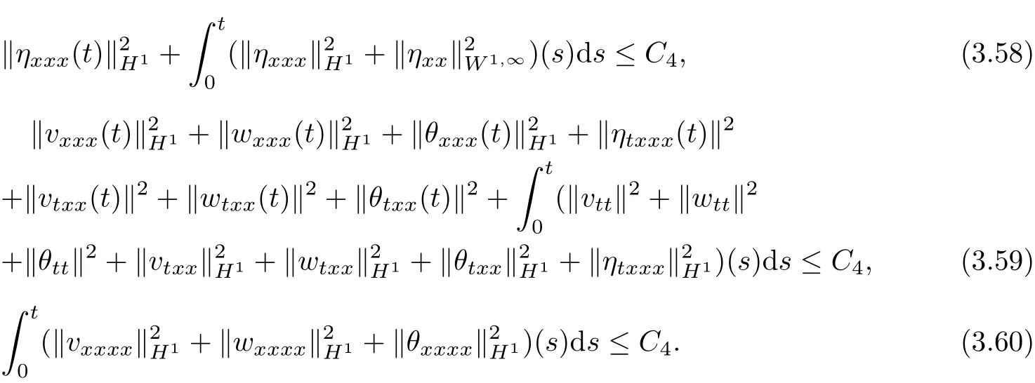
Lemma 3.4 For all t∈[0,T0),there holds:

Proof See,e.g.[24],Lemma 4.3.

Lemma 3.5 For all t∈[0,T0),there holds:

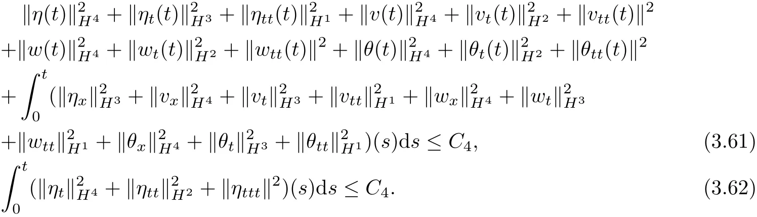
Proof Using(1.1),Lemma 2.1～Lemma 2.4 and Lemma 3.1～Lemma 3.4,we can derive estimates(3.61)～(3.62).The proof is complete.

Proof of Theorem 2 By Lemma 3.1～Lemma 3.5,we have proved the local existence of H4-solution of problem(1.1)～(1.9).

[1]MUJAKOVI´C N.1D compressible viscous micropolar fluid model with non-homogeneous boundary conditions for temperature a local existence theorem[J].Nonlinear Analysis:Real world Applications,2012,13: 1844-1853.

[2]KANEL Y I.Cauchy problem for the equations of gasdynamics with viscocity[J].Siberian Math J,1979, 20:208-218.

[3]OKADA M,KAWASHIMA S.On the equations of one-dimensional motion of compressible viscous fl uids[J]. J Math Kyoto Univ,1983,23:55-71.

[4]QIN Yu-ming,WU Yu-mei,LIU Fa-gui.On the Cauchy problem for a one-dimensionalcompressible viscous polytropic gas[J].Portugaliae Mathematica,2007,64:87-126.

[5]ANTONTSEV S N,KAZHIKHOV A V,MONAKHOV V N.Boundary value problems in mechanics of nonhomogeneous fluids[M].North Holland:Amsterdam,1990.

[6]CHEN Gui-qing.Global solutions to the compressible Navier-Stokes equations for a reacting mixture[J]. SIAM J Math Anal,1992,23:609-634.

[7]CHEN Gui-qing,HOFF D,TRIVISA K.Global solutions of the compressible Navier-Stokes equations with large discontinuous initial data[J].Comm PDE,2000,25:2233-2257.

[8]DAFERMOS C M.Global smooth solutions to the initial boundary value problem for the equations of one-dimensional nonlinear thermoviscoelasticity[J].SIAM J Math Anal,1982,13:397-408.

[9]DAFERMOS C M,HSIAO L.Global smooth thermomechanical processes in one-dimensional nonlinear thermoviscoelasticity[J].Nonlinear Anal,TMA,1982,6:435-454.

[10]DUCOMET B,ZLOTNIK A.Lyapunov functional method for 1D radiative and reactive viscous gas dynamics[J].Arch Rat Mech Anal,2005,177:185-229.

[11]FUJITA-YASHIMA H,BENABIDALLAH R.Unicit´e de la solution de l’´equation monodimensionnelle oua’sym´etrie sph´erique d’un gaz visqueux et calorif´ere[J].Rendi del Circolo Mat di Palermo,Ser II,1993,XLII: 195-218.

[12]FUJITA-YASHIMA H,PADULA M,NOVOTNY A.´Equation monodimensionnelle d´u mgaz vizqueux et calorif´ere avec des conditions initialmoins restrictive[J].Ricerche Mat,1993,42:199-248.

[13]GUO Bo-ling,ZHU Pei-cheng.Asymptotic behavior of the solution to the system for a viscous reactive gas[J].J Diff erential Equations,1999,155:177-202.

[14]JIANG Song.Globally spherically symmetric solutions to the equations of a viscous polytropic idea gas in an exterior domain[J].Comm Math Phys,1996,178:339-374.

[15]JIANG Song.Large time behavior of solutions to the equations of a viscous polytropic ideal gas[J].Ann Mat Pura Appl,1998,CLXXV:253-275.

[16]MUJAKOVI´C N.Globalin time estimates for one-dimensionalcompressible viscous micropolar fl uid model[J]. Glasnik Mathemati´cki,2005,40:103-120.

[17]NAGASAWA T.On the one-dimensional motion of the polytropic ideal gas non-fixed on the boundary[J]. J Differential Equations,1986,65:49-67.

[18]NAGASAWA T.On the the outer pressure problem of the one-dimensional polytropic ideal gas[J].Japan J Appl Math,1988,5:53-85.

[19]NAGASAWA T.Global asymptotic of the outer pressure problem with free boundary[J].Japan J Appl Math,1988,5:205-224.

[20]NAGASAWA T.On the asymptotic behavior of the polytropic ideal gas with stress-free condition[J].Quart Appl Math,1988,46:665-679.

[21]QIN Yu-ming.Global existence and asymptotic behavior for a viscous,heat-conductive,one-dimensional real gas with fi xed and thermally insulated endpoints[J].Nonlinear Anal,TMA,2001,44:413-441.

[22]QIN Yu-ming.Exponential stability for a nonlinear one-dimensional heat-conductive viscous real gas[J].J Math Anal Appl,2002,272507-535.

[23]QIN Yu-ming.Universal attractor in H4for the nonlinear one-dimensional compressible Navier-Stokes equations[J].J Diff erential Equations,2004,207:21-72.

[24]QIN Yu-ming,YU X.Global existence and asymptotic behavior of compressible Navier-Stokes equations for a non-autonomous external force and a heat source[J].Math Meth Appl Sci,2009,32:1011-1040.

[25]MUJAKOVI´C N.Non-homogeneous boundary value problem for one-dimensional compressible viscous micropolar fl uid model:a global existence theory[J].Mathematical Inequalities and Applications,2009,12: 651-662.

tion:35Q30,35M33

1002–0462(2014)01–0129–13

Chin.Quart.J.of Math. 2014,29(1):129—141

date:2013-06-28

Supported by the NNSF of China(11271066);Supported by the grant of Shanghai Education Commission(13ZZ048)

Biography:SUN Lin-lin(1989-),male,native of Zhoukou,Henan,a master candidate of Donghua University, engages in applied partial diff erential equations.

CLC number:O175.29 Document code:A