Wavelet analysis of the hydrological time series of Dalai Lake, Inner Mongolia, China

KeLi Jia , Jian Huang

College of Civil Engineering and Water Resources, Inner Mongolia Agriculture University, Hohhot, Inner Mongolia 010018, China

1 Introduction

Dalai Lake, also called Hulun Lake, is one of the five largest freshwater lakes in China and the largest lake in the Inner Mongolia Autonomous Region. It is located in the Hulunbeir prairie at 48°30′40″N–49°20′40″N and 117°00′10″E–117°41′40″E. The storage of the lake is 13.8 billion cubic meters. When the water level is at 545.55 m, the area of the lake is 2,339 km2, the maximum water depth is 8 m, and the average water depth is 5.7 m. The length of the lake is 93 km, the maximum width is 41 km, and the average width is 25 km. Because the water level dropped by 3.88 m in 2010, the surface area is currently about 1,776 km2. The total area of the Dalai Lake Basin is 202,000 km2, 19.3% of which is in China and 80.7% of which is in Mongolia; about 60% of the surrounding area is prairie land (Figure 1).

The Dalai Lake Nature Reserve is located at the junction of the borders of China, Mongolia, and Russia. This "CMR DAURIA" International Protected Area is designated as a World International Wetland under the Ramsar Wetland Convention, and is also part of the UNESCO Man & Biosphere Nature Reserve network. Current environmental problems at this nature preserve are the shrinkage of Dalai Lake, deterioration of the local ecological environment, biodiversity reduction, and inefficient management under the impacts of climate change and human activities.

The characteristics of the hydrological time series of the Kelulun and Wurxun rivers of the Dalai Lake Basin are analyzed here with wavelet theory to determine their periodicity and variation. Wavelet transform is a multi-resolution analysis method in time and frequency domains, which can spread signals in both domains simultaneously. By flexing and moving operations, functions or signals can be analyzed in detail at multi-scales; here, the properties of different periods of river runoff (wet periods and drought periods) that change with time are studied.

Figure 1 Location of the Dalai Lake Basin

The wavelet theory was introduced into hydrology research in the late 20th century. Wavelet theory was utilized by Jean Morlet and Alex Grossman when they analyzed earthquake data in 1981 (Merry, 2005), and it was first used in hydrology by Kumar and Foufoula-Georgiou in 1993.The orthogonal wavelet (Haar wavelet) is often used to study the scale of spatial precipitation and oscillation characteristics; results have shown that they exhibit self-similar behavior over a wide range of time scales (Kumar and Foufoula-Georgiou, 1993). Wavelet package analysis was used by Venckp and colleagues to do wavelet decomposition in 1996; they identified the time-frequency scale which led to a new understanding of precipitation-forming mechanisms (Venckp and Foufoula-Georgiou, 1996). The multi-time-scale structure of the precipitation of Xi’an City over the last 50 years was analyzed by ZiWang Deng and colleagues in 1997 based on the Morlet wavelet transform(Deng and Lin, 1997). The chaos wavelet network model,which combines wavelet analysis, chaos theory, and artificial neural networks (ANNs) was developed by YongLong Zhao and colleagues in 1998, was used to make long-term predictions of daily flow series of the Jinshajiang River at Pingshan station, and the results showed that the model is more optimal than the multi-variable regression model(Zhao and Ding, 1998). The Marr wavelet transform was used to analyze the multi-scale time structure of rainfall before and after the flood season, as well as the annual rainfall,of Guangzhou in 1999 (Ji and Gu, 1999), and the wavelet transform was used by Xian Deng and colleagues to determine the implicit periods of hydrological time series based on the physical occurrence of hydrological phenomena(Deng and Zhang, 1999). A coupled prediction model using ANN and wavelet transform was developed by XianBin Li and colleagues, wherein the wavelet transform is first used for the hydrological time series and then the ANN model is applied to do multi-scale combined prediction with the wavelet transform coefficients, and the original hydrological series is reconstructed for the prediction (Li and Ding, 1999).Sun (2000) used the wavelet transform to analyze the abnormal conditions of summer precipitation in the northeast part of China, and Jing (2000) developed a multi-step prediction model coupling ANN and wavelet analysis for meteorological modeling. Wang and Ding (2003) used Marr and Morlet wavelets to transform a 100-year average annual flow series of the Yangtze River at Yichang station, and conduct a multi-scale time analysis.

2 The basic environmental conditions of the Dalai Lake Basin

The study area is part of the Dalai Lake Basin in China(Figure 1). The climate of the Dalai Lake Basin is a semi-arid temperate continental climate in a high altitude.Winter is cold and very harsh from October until following May; spring is windy from May to the end of June; summer is cool from the end of June to the beginning of August with rainfall, and fall extends from the beginning of August to early October.

2.1 Temperature

We analyzed the 1958–2007 weather data of three weather stations around Dalai Lake. The annual average temperature is 0.24 °C, the lowest temperature is -22.58 °C in January, and the highest temperature is 20.34 °C in July.The average annual temperatures are shown in Figure 2. The variation of the average monthly temperature is shown in Figure 3.

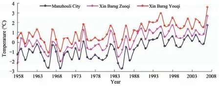
Figure 2 Annual temperature

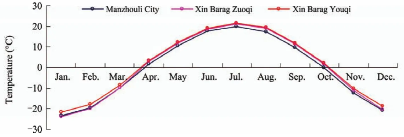
Figure 3 Mean monthly temperature

2.2 Precipitation

The average annual precipitation of the Dalai Lake Basin is 264.3 mm; the annual precipitation is shown in Figure 4 and the average monthly precipitation is shown in Figure 5.The average snow depth of Dalai Lake varies from 3.8 cm in the east to 2.06 cm in the west, and the average annual snow depth is shown in Figure 6.

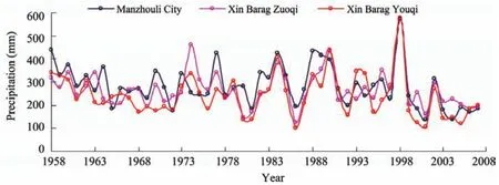
Figure 4 Annual precipitation

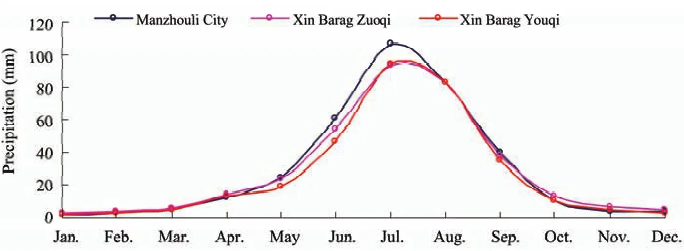
Figure 5 Average monthly precipitation

Figure 6 Annual average snow depth

2.3 Wind

The average wind speed is 3.75 m/s, and the northwest wind is predominant in the basin. The annual wind variation and average monthly wind speed are shown in Figures 7 and 8.

2.4 Sunshine

The average annual daily sunshine is 8.18 hours; the average annual and monthly daily sunshine hours are shown in Figures 9 and 10.

2.5 Evaporation

The average annual evaporation is 1,669.9 mm; the annual and monthly evaporation are shown in Figures 11 and 12.

2.6 Hydrological characteristics of the Dalai Lake Basin

The Kelulun and Wurxun rivers are the main inflow to Dalai Lake. The Wurxun River flows from Beir Lake to Dalai Lake and accepts flow from the Halaha River. Its length is 223 km and it is the most important channel for fish spawning between Beir Lake and Dalai Lake. Wulan Pond is located 80 km south of Dalai Lake; it is also an important wetland for fish spawning and bird habitat. The annual average flow volume of the Wurxun River is 2.171×108m3.The Kelulun River originates in the Khenti Mountains in Mongolia; its length is 1,264 km, 206 km of which is in China. Its annual average flow volume is 5.367×108m3. The annual flow volume and the minimum, maximum, and average monthly flow volume of the two rivers are shown in Figures 13 and 14.

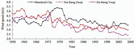
Figure 7 Average annual wind speed

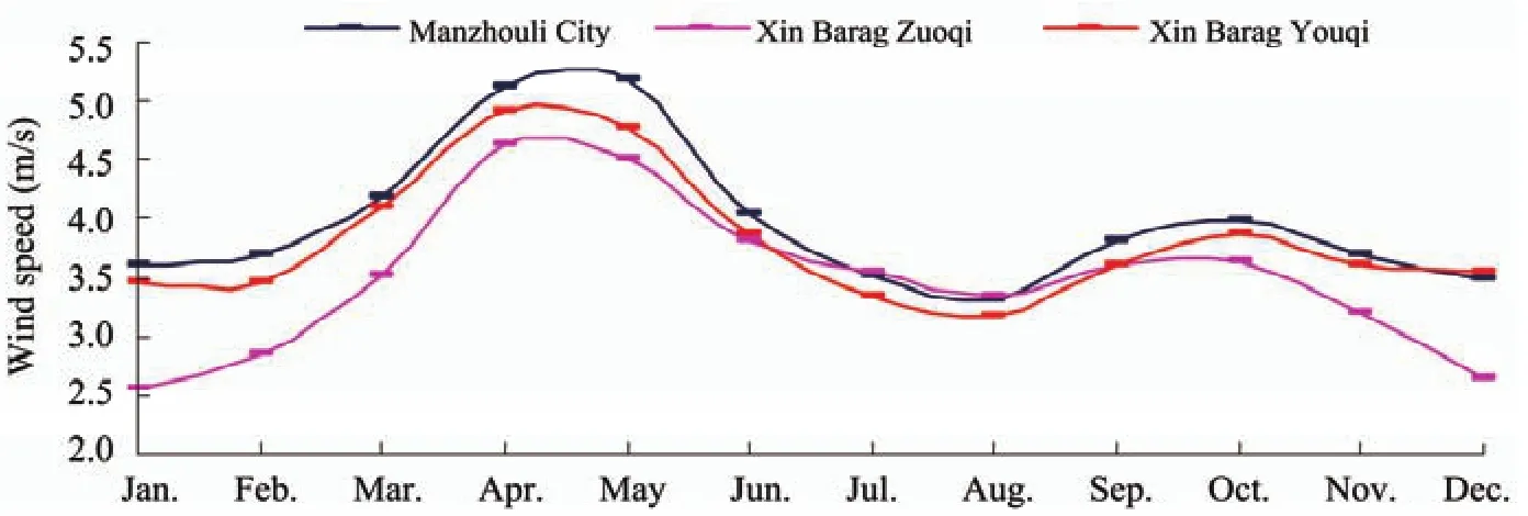
Figure 8 Average monthly wind speed

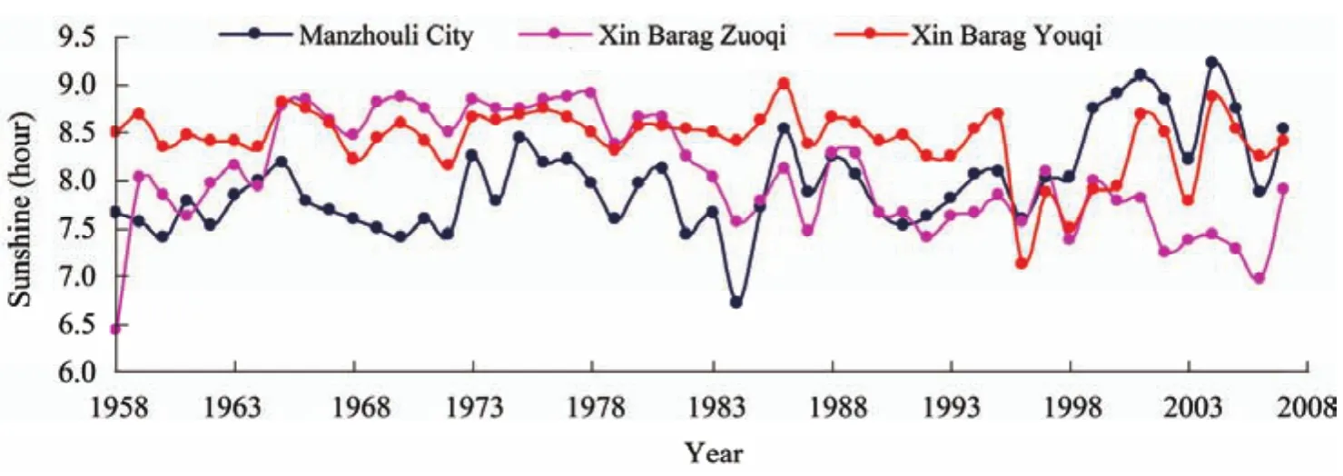
Figure 9 Average daily sunshine

Figure 10 Average monthly daily sunshine

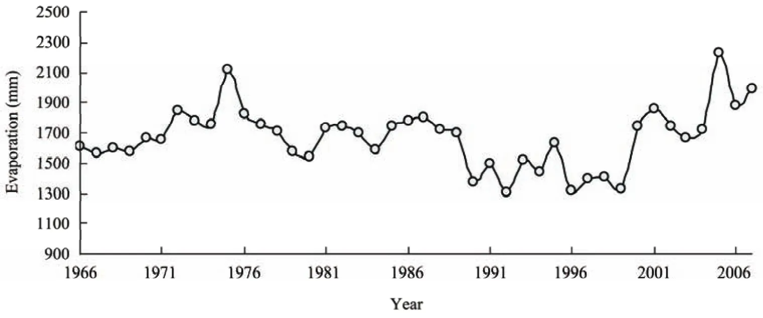
Figure 11 Average annual evaporation

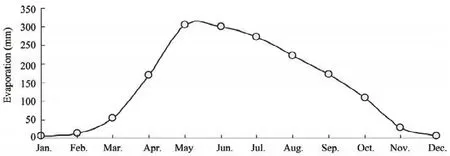
Figure 12 Mean monthly evaporation

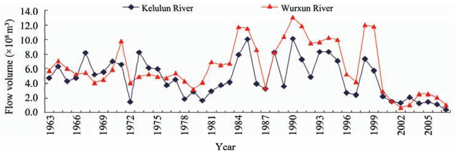
Figure 13 Annual average flow volume of Kelulun (blue) and Wurxun (red) rivers

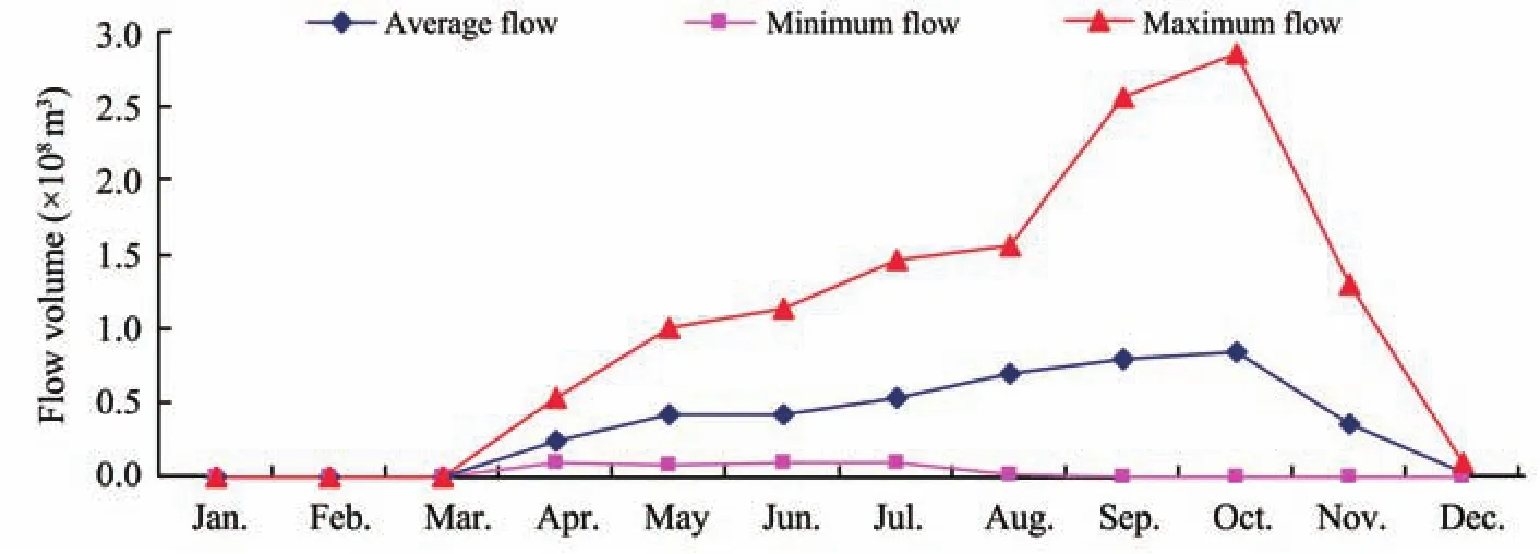
Figure 14 Average, minimum and maximum monthly flow of Kelulun and Wurxun rivers

Figure 13 shows that the high and low flow trends of the two rivers are basically the same. Their flow volumes were about 500 million cubic meters and 200 million cubic meters annually from 1963 to 1980, but have declined to less than 200 million cubic meters annually from 2000 until now. The Wurxun River ceased to flow in 2008. However, the monthly flow volume variation of the two rivers is significantly different. The highest flow volume of the Kelulun River is in October, whereas the highest flow volume of the Wurxun River is in August. The annual water level of Dalai Lake in August is shown in Figure 15; the water level began to drop dramatically after 2000, at a rate of 0.4 m/a. The relationship of the lake’s open water area and water level is shown in Figure 16.

There are several seasonal streams and ponds in the Dalai Lake Basin that depend on the yearly precipitation. The water quality of Dalai Lake is good, ranked as type 3, and the water quality of the Wurxun and Kelulun rivers is also good, ranked as type 2 in accordance with the National Surface Water Quality standard for drinking.

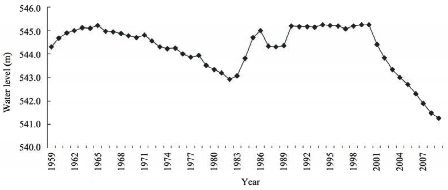
Figure 15 Average water level of Dalai Lake in August

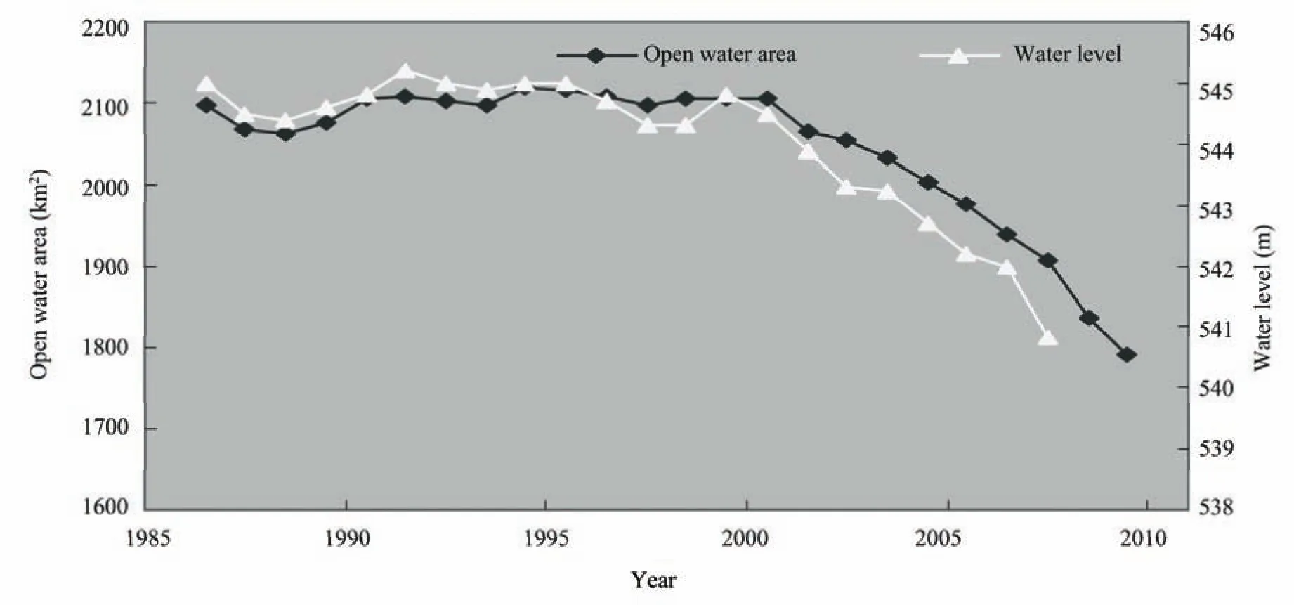
Figure 16 Water level and open water area of the Dalai Lake

3 Complexity analysis of the hydrological time series of the Dalai Lake Basin

Wavelet analysis is here combined with complexity theory to study the complexity and the multi-time-scale characteristics of the hydrological series of Dalai Lake. This includes calculation of the wavelet transform coefficient of the hydrological series, fractal calculations based on discrete wavelet transforms, and wavelet denoising of the hydrological series.

3.1 Continuous wavelet transform

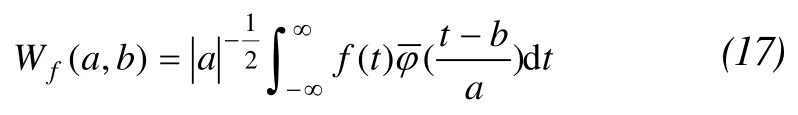
A continuous wavelet transform (CWT) is performed via the translation and dilation (or contraction) of a mother waveletφ(t) across the seriesf(t) as a function of timet.SupposeL2(R) is the measurable quadratic integrable function. If the functionf(t)∈L2(R) satisfies:

then the function can be used to represent the continuous time signal or the modeling signal of limited power. For the signalf(t)∈L2(R), the continuous wavelet transform (CWT)is defined as:

whereWf(a,b) is the wavelet transform coefficient,φ(t) is the basic wavelet or mother wavelet, < > is the inner product,ais the scale coefficient,bis the time shift coefficient, andφa,b(t) is the continuous wavelet:

The basis is called a "wavelet" basis and consists of all the translated and dilated versions of the "mother" wavelet.

3.2 Discrete wavelet transform

In nature, observed hydrologic series are usually discrete signals, so the parametersaandbare discretized and then the discrete wavelet transform (DWT) is performed as:a=,b=,a0>0 anda0≠ 1,b0∈R.

whereZis an integer, the discrete wavelet transform off(t) is:

3.3 Wavelet denoising procedure

We used a wavelet denoising method based on thresholds for acquiring correct denoised results. This method,which is now the most common method of wavelet denoising, is performed as follows:

(1) Choose an appropriate mother wavelet and number of resolution level,N. The original one-dimensional time series is decomposed into an approximation at resolution levelNand detailed signals at various resolution levels by using the wavelet transform.

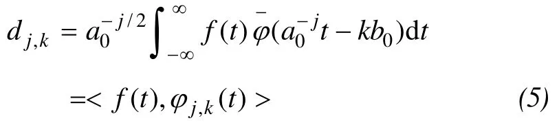
(2) As a soft threshold process, below certain thresholds the absolute values of detailed signals,dj(t) (j= 1, 2, ...,N)are set to zero at each resolution level. The subscriptjrepresents thejth resolution level. The absolute values of the detailed signals that exceed certain thresholds are treated as the difference between the values of the detailed signals and the thresholds as follows:

The thresholdTis defined as Stein’s unbiased risk threshold:

whereδis the noise intensity, andW=[w1,w2, …,wn],w1≤w2≤…≤wnis the wavelet coefficient series.

The risk vectorR=[r1,r2, …,rn] is calculated, and

The minimum valuerbofRis the risk value, and the correspondentwbis determined. Equation(6)gives the threshold quantifications used to obtain the processed detailed signals at each resolution level during wavelet denoising. The approximation usually does not perform threshold quantifications.

(3) Wavelet reconstruction can derive the denoised time series data from the approximation at resolution levelNand the processed detailed signals ()(ˆtdj) at all resolution levels.

3.4 Fractal estimation of the hydrological series based on CWT

The underlying principle of fractals is that a simple process that goes through infinitely many iterations becomes a very complex process. Fractals attempt to model the complex process by searching for the simple process underneath.Most fractals operate on the principle of a feedback loop. A simple operation is carried out on a piece of data and then fed back in again. This process is repeated infinitely many times. The limit of the process produced is the fractal. Almost all fractals are at least partially self-similar. This means that a part of the fractal is identical to the entire fractal itself except smaller. Fractals can look very complicated, but usually they are very simple processes that produce complicated results. This property transfers over to chaos theory, wherein if something has complicated results, it does not necessarily mean that it had a complicated input. Chaos may have crept in (e.g., in something as simple as a round-off error in a calculation), producing complicated results. Fractal dimensions are used to measure the complexity of objects, providing ways of measuring things that were traditionally meaningless or impossible to measure.

3.4.1 Statistical self-similarity of the hydrologic series

X(t) is a stochastic hydrological series; for anya>0,there is:

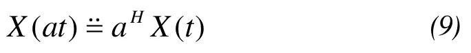
X(t) is a statistical self-similarity, whereHis the self-similarity coefficient or Hurst coefficient, =˙˙ is the probability distribution equality, andais scale. The mean,autocorrelation, and power spectrum of a self-similarity process are all of self-similarity. For a statistical self-similarity processX(t), the relationship of the spectral density functionSand the angular frequencyωis:

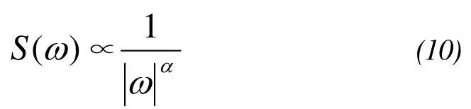
whereαis the frequency spectrum index, -1<α<3. When 1<α<3,α= 2H+1,X(t) is fractional Brownian motion; when-1<α<1,α= 2H-1, thenX(t) is the fractional Gaussian noise.In practical terms,ωis meaningful only when it is a positive number.

3.4.2 α estimation formula based on wavelet analysis

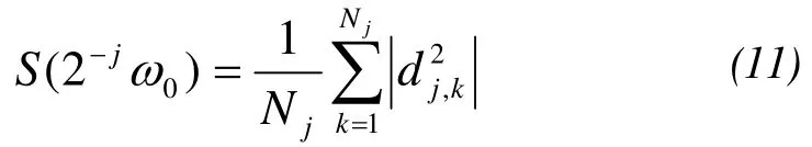
Wavelet transform is used to a hydrological series {X(t),t= 1, 2, …,N}, the transform coefficient isdj,k. Theαestimator is deduced with the frequency spectrum. The basic wavelet function is of the vanishing momentR(≥α/2) . The energy spectrum of the wavelet transform coefficientdj,kat 2-jω0(ω0is the reference frequency of the basic wavelet function) is:

Based on the frequency spectrum of the statistical self-similarity process, there is:

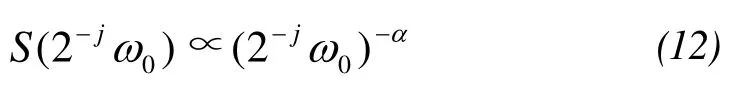
wherec0is a constant.

3.4.3 Estimation procedure of the fractal D based on the wavelet analysis

(1) Calculate the wavelet transform coefficientdj,k:

For a given stochastic hydrologic seriesX(t), the multi-resolution orthogonal Daubechies (DbN) wavelets are selected; thedj,kisajcalculated by the Mallat fast wavelet transform.aj(j= 1, 2, …,M;Mis the maximum decomposition number).

(2) The logarithm of the power spectrum of the wavelet transform coefficient atjis:

(3) The least squares estimation of the regression coefficients of the regression equation is used to get the frequency spectrumα:

The fractal dimensional values of the hydrological series are:

4 Fractal estimation of the annual flow volume of the Dalai Lake Basin

4.1 Annual flow volumes of the Kelulun and Wurxun rivers

We used the annual flow volumes of the Kelulun and Wurxun rivers from 1963 to 2007. We selected the orthogonal wavelet DbNs and decomposed the annual flow volume series in six levels, with DbNs established by the Malltat method. The wavelet decomposition coefficients Db5 of the two rivers are shown in Figure 17.

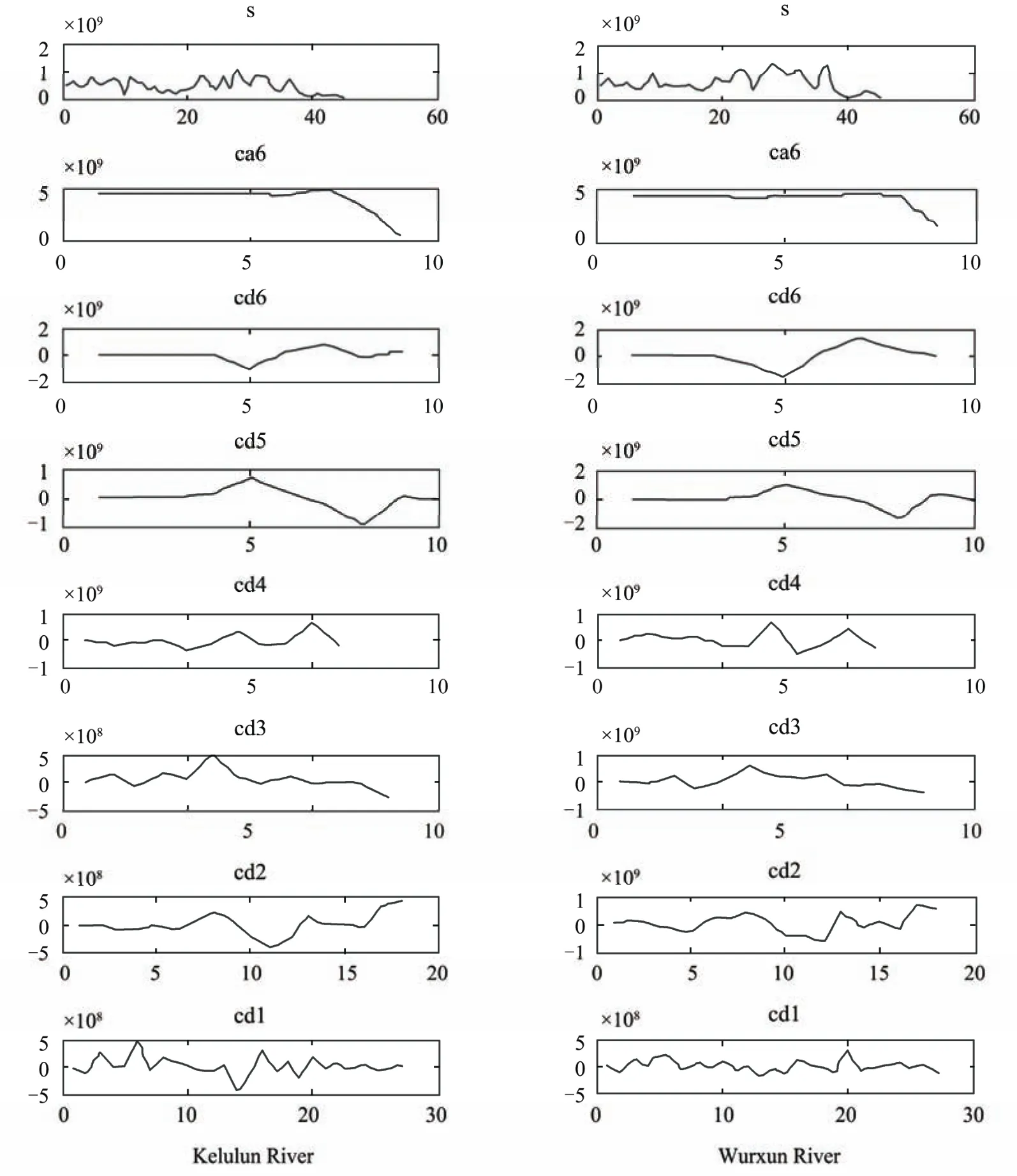
Figure 17 Annual runoff hydrological sequences’ wavelet coefficients Db5 wavelet

The fractals (D) correspondent to the DbNs of different vanishing moments of the Kelulun and Wurxun rivers are shown in Tables 1 and 2. The regression equations correspond to the different DbN wavelets that are shown in Figures 18, 19, and 20.

It can be seen from Table 1 that the fractals Db3, Db4,Db5 tend to be stable as 1.183, 1.158, and 1.186, respectively. The regression equation of Db5 has the higher fit precision, withR2=0.876. Hence, the fractal value of the annual flow volume of the Kelulun River is 1.186 with the Db5 wavelet. It can be seen from Table 2 that the fractal values are 1.015 and 1.019, calculated with Db4 and Db5,and are stable. The regression equation of Db5 has the higher fit precision, withR2=0.816. Thus, the fractal value of the annual flow volume of the Wurxun River is 1.019 with the Db5 wavelet. The calculation results show that the fractal value of the Kelulun River is 1.186, larger than the 1.019 of the Wurxun River; hence, the variation of the annual hydrological process of the Kelulun River is more intense than that of the Wurxun River.

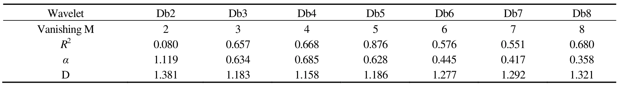
Table 1 Annual runoff of the Kelulun River: fractal dimensions are extracted by DbN wavelets of different vanishing moments

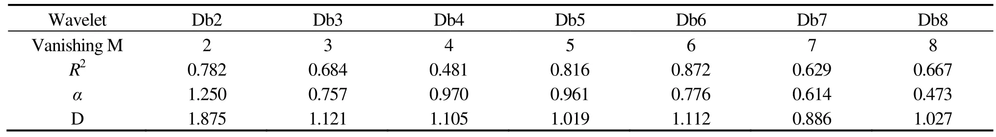
Table 2 Annual runoff of the Wurxun River: fractal dimensions are extracted by DbN wavelets of different vanishing moments

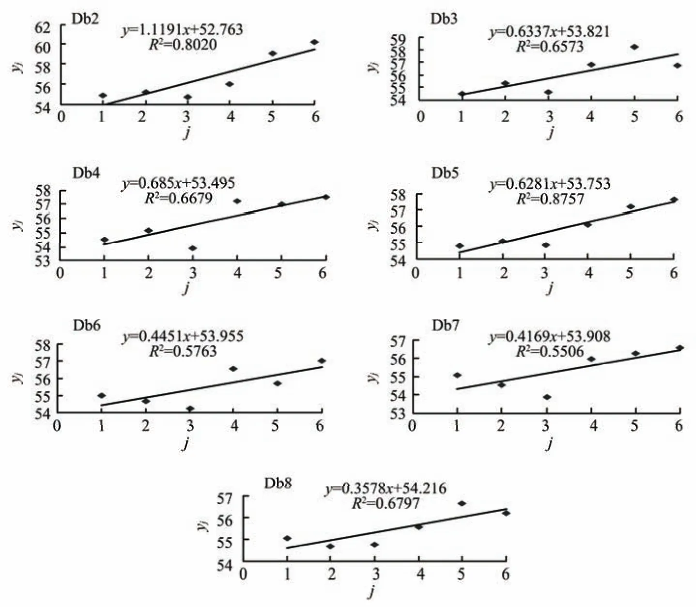
Figure 18 Regression equations by different DbN wavelets in the Kelulun River

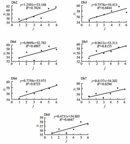
Figure 19 Regression equations by different DbN wavelets in the Wurxun River

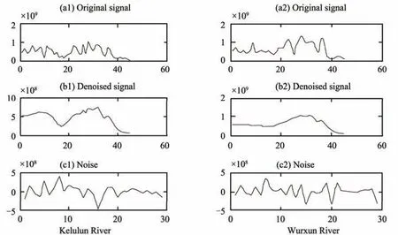
Figure 20 Denoising of annual runoff

4.2 Fractal estimation of the annual flow volumes after denoising

Through many attempts with different decompositions of wavelets, we found that the sym7 wavelet had better symmetry to do three decompositions of the hydrological series. We used the Stein soft threshold to do the denoising; the original properties of the signal were preserved with proper denoising.

The estimation results of the Kelulun and Wurxun rivers before and after denoising showed that the variation of the annual flow volume series of Kelulun River oscillated more than that of the Wurxun River (Tables 3 and 4). The regression equations of different DbN wavelets of the annual flow volume series after denoising had higher fitting precision(Figures 21 and 22 ); theR2was larger than that of the series before denoising and they were also quite stable. The fractal values (D) of the Kelulun and Wurxun rivers were larger after denoising compared with those before denoising,which shows that noise interfered with the original hydrological series, and the complexity was also small. Thus, the real complexity can be determined by the results after denoising, which were larger than those before denoising.

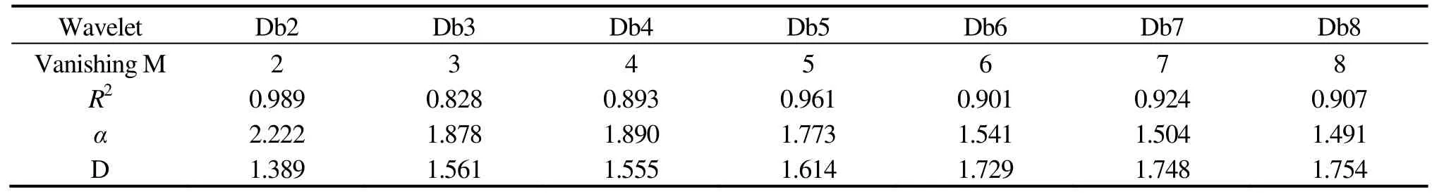
Table 3 Annual runoff of the Kelulun River: fractal dimensions are extracted by denoising DbN wavelets of different vanishing moments

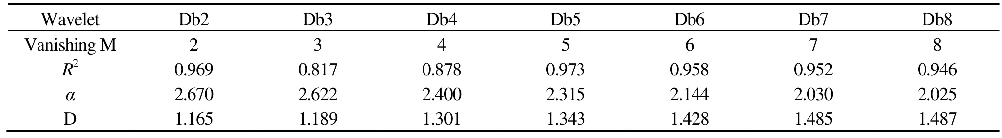
Table 4 Annual runoff of Wurxun River: fractal dimensions are extracted by denoising DbN wavelets of different vanishing moments

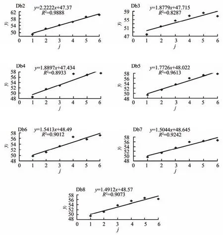
Figure 21 Regression equations by different DbN wavelets after denoising the hydrological sequence of the Kelulun River

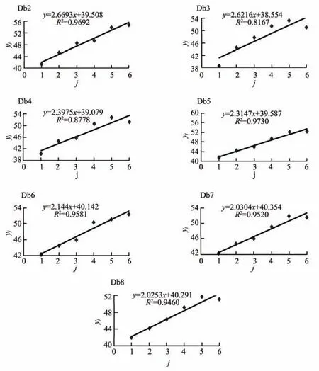
Figure 22 Regression equations by different DbN wavelets after denoising the hydrological sequence of the Wurxun River

4.3 Fractal estimation of the monthly flow volumes of the Kelulun and Wurxun rivers

We used data from 540 monthly flow volume series spanning 45 years of the Kelulun and Wurxun rivers for analysis. We used the orthogonal DbN wavelets to do six level decompositions with Mallat fast calculations, as shown in Figure 23 using Db4 as an example.

The fractal values (D) corresponding to different vanishing moments of the Wurxun and Kelulun rivers are shown in Tables 5 and 6.

4.4 Fractal estimation of the monthly flow volumes after denoising

The sym6 wavelets, which had better symmetry, were used to do three decompositions of the monthly flow volume series. The hydrological series maintained the significant regularity of the original properties after denoising.

The fractal values calculated with different DbNs of monthly and annual flow volume of the Kelulun River were all larger than those of the Wurxun River, and the results were consistent with the series before and after the denoising. Hence, the variations of both monthly and annual flow volume series of the Kelulun River were more complex than those of the Wurxun River, and the variation of the monthly flow volume series of the Kelulun River was more complex than that of the annual flow volume series of the Kelulun River. The variations of monthly flow volume and annual flow volume of Wurxun River were similar to those of the Kelulun River (Figures 24 and 25,Tables 7 and 8).

5 Application of wavelet analysis in a multiple time-scale analysis of the hydrological system

A multiple time scale of a time series describes a system that does not have meaningful periodicity, but has variant periods with different time scales in the same time span.There are multiple-time-scale structures and local variation characteristics. The study of a multiple time scale will determine the development trend and regular pattern of the system in different time scales, so that medium- and long-term predictions of the system can be achieved.

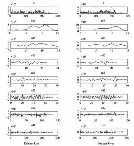
Figure 23 Monthly runoff hydrological sequences’ wavelet coefficients under six decomposition by Db4 wavelet

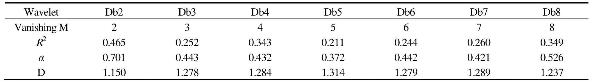
Table 5 Monthly runoff of the Kelulun River: fractal dimensions are extracted by DbN wavelets of different vanishing moments

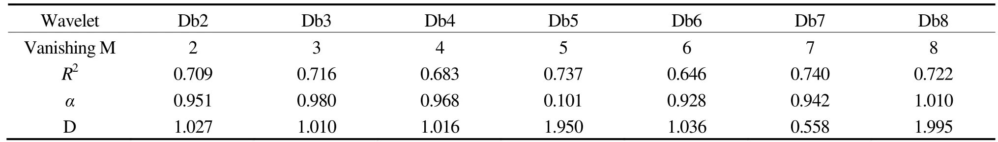
Table 6 Monthly runoff of the Wurxun River: fractal dimensions are extracted by DbN wavelets of different vanishing moments

The fractal value (D) of the Kelulun River was 1.284 withR2= 0.343; the fractal value (D) of the Wurxun River was 1.016 withR2= 0.683.

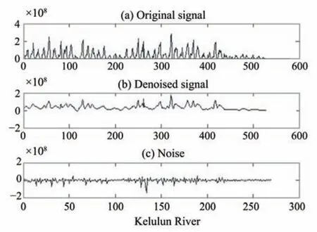
Figure 24 Denoising of the Kelulun River’s monthly runoff

Figure 25 Denoising of the Wurxun River’s monthly runoff

Table 7 Monthly runoff of the Kelulun River: fractal dimensions are extracted by denoising DbN wavelets of different vanishing moments

5.1 The wavelet transform coefficient chart

For a given wavelet functionϕ(t), the continuous wavelet transform of )()(2RLtf∈ is:

whereais a scale factor that represents the period length of the wavelet,bis the time factor reflecting the time shift, andWf(a,b) is the wavelet transform coefficient that varies withaandb. Ifbis the horizontal ordinate andais the vertical axis, then theWf(a,b) plot is called a wavelet transform coefficient chart.

5.2 Wavelet variance

The wavelet variance is defined as the integral of any wavelet coefficient of different time scales in the time domain. The equation is:

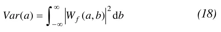
whereVar(a) is the wavelet variance and a refers to the time scale. The dominant time scales of a certain time series,namely, the significant periods, will be verified through tests of wavelet variance.

5.3 The variable characteristics of a multiple-time structure of the annual flow series

5.3.1 The annual flow series of the Kelulun River

The variable characteristics of a multiple-time structure of the annual flow series of the Kelulun River (45 years of annual flow volume data from the Alatanmole hydrological gauge station) were standardized to study the multiple-time-scale properties with a Morlet wavelet transform(Figure 26).

The wet and drought patterns of annual runoff in different time scales were clearly shown in the time-frequency structure figure of the wavelet coefficient. The inter-annual and inter-decadal variations at scales of 1–7 years and 7–12 years are very apparent in Figure 27a. The real part of the Morlet wavelet transform coefficient of the standardized series of the Kelulun River is shown in Figure 27b, which clearly shows the time-scale variation, the abrupt changes at time different scales, and the phase structure of the annual flow volume series. The wet characteristics of the annual flow volume series in the periods 1963–1968, 1973–1978,1983–1987, and 1992–1996 are the positive phase, while the drought characteristics of the annual flow in the periods 1968–1973, 1978–1983, 1987–1992, and 1996–2000 are the negative phase. The abrupt changes in 1968, 1973, 1977,1982, 1986, 1996, and 2001 are in the years when transition between wet and drought occurred.

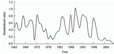
Figure 26 Standardization process of annual runoff in Kelulun River

The inter-decadal variation of 20–30 years is significant,with the center at 25 years. The variation process of the wavelet transform coefficient at the 25-year scale is shown in Figure 28c. The annual flow of the Kelulun River is characterized as wet in 1963–1975 and 1987–2000,drought in 1975–1987 and after the year of 2000, and the abrupt changes in 1975, 1987, and 2000 occurred during transitions between wet and drought periods. Therefore,the Kelulun River has been in a drought period since 2000;given that 25 years is the full period and that there is a cycle of wet and drought periods every 12 years, it is predicted that the Kelulun River will gradually transition into a wet period after 2012.

The main 11-year and 24-year periods years of the wavelet variance of the Kelulun River annual flow series are shown in Figure 29, and are consistent with the results of the above analysis. Hence, the main periods of the annual flow series of the Kelulun River are 10 and 25 years.

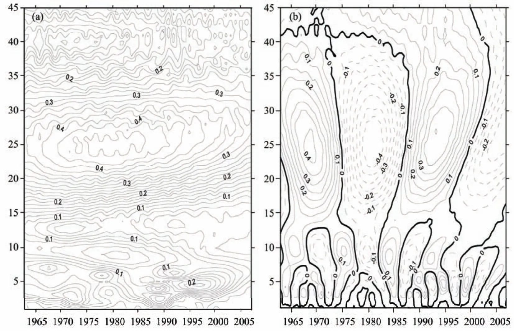
Figure 27 Time-frequency structures of the modulus (a) and the real part of the Morlet wavelet (b)

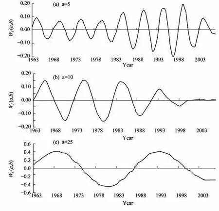
Figure 28 The real progress of change annual runoff in Kelulun River

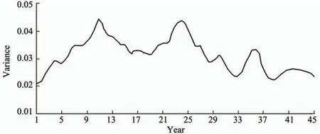
Figure 29 The wavelet variance of annual runoff in Kelulun River

5.3.2 The annual flow series of the Wurxun River

A similar analysis of 45 years of annual flow data for the Wurxun River (from the Kuduleng hydrological gauge station) is shown in Figures 30, 31, and 32.

The inter-annual variation at the 1–10 year scale of the time-frequency structure of the Morlet wavelet transform coefficient plane of the Wurxun River (Figure 31a) is obvious in the period from 1981 to 2007; the oscillation center is in 1994. The inter-decadal variation at the 18–32 year scale is obvious and mainly occurs in the period of 1963–2007;the oscillation center is in 1990. The time scale, the abrupt changes, and the phase structure of the real part of the Morlet wavelet transform coefficient time-frequency are shown in Figure 31b. The inter-annual variation at the 1–10 year scale is obvious, with the center at 8 years and the positive and negative phases occurring in turn. The inter-decadal variation at the 18–30 year scale is also obvious, with the center at 25 years. The wet periods of 1963–1973 and 1986–2000 show the positive phase, and the drought periods of 1973–1986 and after 2000 show the negative phase,which is similar to that of the Kelulun River,i.e., 25 years of wet and drought periods. The 25-year cycle of wet and drought periods is clearly shown in the wavelet variance plot in Figure 33. The wet and drought cycles of the Kelulun and Wurxun rivers are the same, 25 years, and it is predicted that the Wurxun River will enter a wet period gradually after 2012.

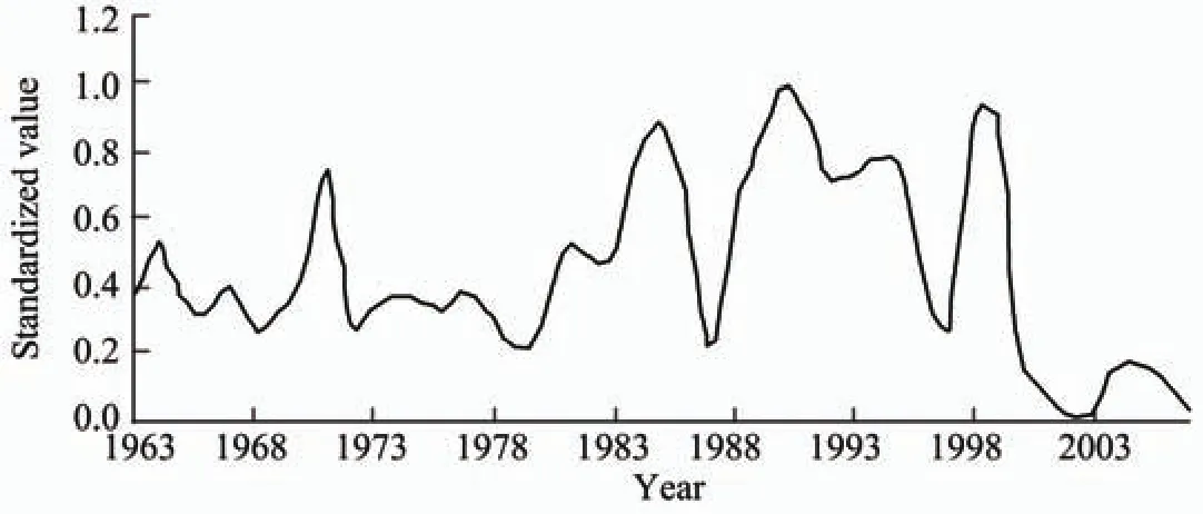
Figure 30 Standardization process of annual runoff in the Wurxun River

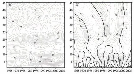
Figure 31 Wavelet transform coefficients modulus (a) and the real time-frequency distribution (b) of annual runoff in the Wurxun River

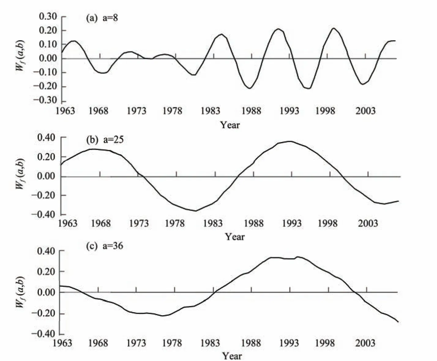
Figure 32 The real process of changes in annual runoff in the Wurxun River

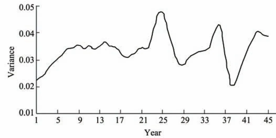
Figure 33 The wavelet variance of annual runoff in Wurxun River

5.3.3 The monthly flow series of the Kelulun and Wurxun rivers

The monthly flow volume series of the Kelulun and Wurxun rivers from 1963 to 2007 were used to do the analysis. The results are shown in Figures 34, 35, 36, and 37.The results show that there is a 320-month period of wet and drought. There is wet and drought variation every 160 months, and the two rivers have the same wet and drought cycle of 25 years.

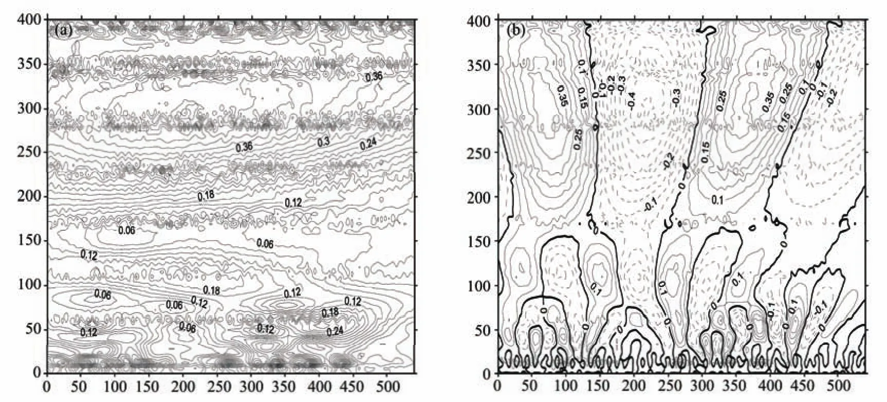
Figure 34 Wavelet transform coefficients modulus (a) the real time-frequency distribution (b) of monthly runoff in the Kelulun River

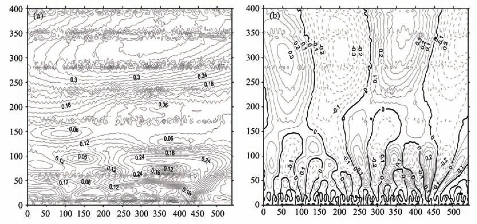
Figure 35 Wavelet transform coefficients modulus (a) the real time-frequency distribution (b) of monthly runoff in the Wurxun River

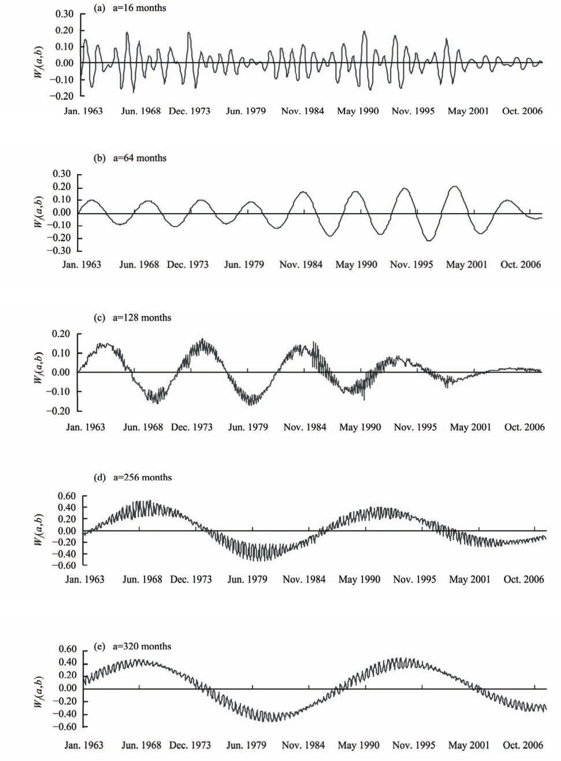
Figure 36 The real process of changes in monthly runoff in the Kelulun River

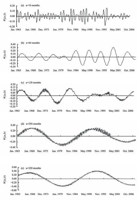
Figure 37 The real process of changes in monthly runoff in the Wurxun River

6 Conclusion

Wavelet theory is used to analyze the hydrological time series of the Kelulun and Wurxun rivers in the Dalai Lake Basin. The flow volume variation processes of the Kelulun River in different years and months are more complex than those of the Wurxun River. The monthly hydrological complexity of the two rivers is greater than that of the annual hydrological complexity. Db5 wavelets proved to be more appropriate for the wavelet computation of the annual flow volume of the Dalai Lake watershed, whereas Db4 wavelets were more appropriate for the wavelet computation of the monthly flow volume.

Wavelet analysis is also used to analyze the multiple-time-scale structure and abrupt changes in the Kelulun and Wurxun rivers. The results show that the two rivers have similar variation, and there is a 25-year cycle of wet and drought periods,i.e., wet and drought cycles every 12 years.Because the Kelulun and Wurxun rivers are the two main rivers in the Dalai Lake Basin, the multiple-time-scale variation of the hydrological series of these two rivers represents the variation of the Dalai Lake Basin. The periods 1963–1975 and 1987–2000 were wet periods, and 1975–1987 and after 2000 were the drought periods in the Dalai Lake Basin. Abrupt changes occurred in 1975, 1987,and 2000, which were transitions between wet and drought.The Dalai Lake Basin has been in drought since 2000, and it is predicted that it will gradually transit to a wet period after 2012. The current rapid shrinkage of Dalai Lake is directly related to the drought period after 2000.

The author is grateful to Dr. Ramasamy Jayakumar for his inspiring and support. The paper is supported by the project"Ecohydrological process modeling of Dalai Lake Basin under different grazing system" granted by the National Natural Science Foundation of China (Grant No. 51169011).

Deng X, Zhang WS, 1999. The approximate period determination of hydrological series based on wavelet analysis. Hydrology, 6: 22–25.

Deng ZL, Lin ZS, 1997. Multiple time scale analysis of the 50 years of climate change in Xi’an City. Plateau Meteorology, 16(1): 81–93.

Ji ZP, Gu DJ, 1999. Multiple time scale analysis of 100 years of climate in Guangzhou. Tropical Meteorology, 5: 48–55.

Jiang XH, Liu CM, 2003. The driving and multiple time scale variation of natural runoff of upper and medium reaches of Yellow River. Natural Resources, 18(2): 142–147.

Jing L, 2000. Multiple step prediction of wavelet ANN coupling model.Atmosphere Science, 24(1): 71–86.

Kumar P, Foufoula-Georgiou E, 1993. A multi-component decomposition of spatial rainfall fields, 1. Segregation of large and small scale features using wavelet transforms. Water Resources Research, 29(8): 2515–2532.

Li XB, Ding J, 1999. ANN network prediction based on the reconstructed series of wavelet transform. Water Resources, 2: 1–4.

Merry RJE, 2005. Wavelet Theory and Applications: A Literature Study.Eindhoven University of Technology, Department of Mechanical Engineering, Eindhoven, The Netherlands, pp. 9.

Sun L, 2000. Climate analysis of summer abnormal rainfall in northeast part of China. Meteorology, 58(1): 72–80.

Venckp V, Foufoula-Georgiou E, 1996. Energy decomposition of rainfall in the time-frequency-scale domain using wavelet packets. Journal of Hydrology, 187: 3–27.

Zhao YL, Ding J, 1998. The application of the chaos wavelet network model in the medium to long term predication of hydrology. Development of Water Science, 9(3): 252–257.