Precipitation-runoff simulation for a Himalayan River Basin,India using artificial neural network algorithms

Ray Singh Meena, Ramakar Jha , Kishanjit Kumar Khatua

Department of Civil Engineering, National Institute of Technology, Rourkela, India

1 Introduction

The precipitation-runoff relationship is an important issue in hydrology and a common challenge for hydrologists. Due to tremendous spatial and temporal variability of Himalayan Basin characteristics, such as snow pack, land use/land cover, soil moisture, hydraulic conductivity, topography (relief), and erratic rainfall for example, the precipitation-runoff relationship is usually considered as a nonlinear process. Since the middle of the 19th century,different methods have been demonstrated by hydrologists for precipitation-runoff modeling whereupon many models have attempted to describe the physical processes involved(e.g., mathematical, physical, lumped or distributed models).

Over the last decade, there has been a tremendous growth in the application of a class of techniques that operate in a manner analogous to that of biological neurons system,i.e.,Artificial Neural Networks (ANNs). While ANNs are capable of capturing non-linearity in the precipitation-runoff process compared with other modeling approaches (Hsuet al., 1995).ANN models have been applied in hydrology in the context of precipitation-runoff modeling (Dawson and Wilby, 1998;Tokar and Markus, 2000; Zhang and Govindaraju, 2003;Kumaret al., 2005), runoff analysis in humid forest catchment(Elshorbagyet al., 2000), river flow prediction (Gautamet al.,2000; Garcia-Bartual, 2002), setting up stage-discharge relations (Harunet al., 1996), and short term river flood forecasting (Imrieet al., 2000). From these studies, it has been established that ANN models can be flexible enough to successfully simulate precipitation-runoff processes.

ANN is an information-processing system composed of many nonlinear and densely interconnected processing ele-ments or neurons. Each neuron is linked to its neighbours with an associated weight that represent information used by the net to solve a problem. Neurons are arranged in groups called layers and operate in logical parallelism. Information is transmitted from one layer to others in serial operations.Three basic layers of ANNs are the input, hidden and output layers. Various types of neural network models are available for precipitation-runoff modeling. Feed Forward Artificial Neural Networks (FFANNs) maintain a high level of research interest due to their ability to map any function to an arbitrary degree of accuracy. This has been demonstrated theoretically for both the Radial Basis Function (RBF) network and the Popular Multilayer Perceptron (MLP) network(Harpham and Dawson, 2005). The primary goal of ANN modeling is the prediction or forecasting of hydrological variables,e.g., runoff prediction.

In the present work, different types of ANN algorithms were used for precipitation-runoff modeling for three discharge measuring stations (Barahkshetra, Bhimnagar and Baltara) of the Himalayan Kosi Basin using monsoon data for the years of 2005–2009. The data was divided into three sets prior to building the ANN model: the training,testing and validation sets. The validation set was kept aside to evaluate the accuracy of the model derived from the training and testing sets. The model performance was evaluated using global statistics and non-parametric tests.

2 The study area and data collection

The Himalayan Kosi Basin is an integral part of the Ganga River System, with the upper portion lying in Nepal and Tibet in the Himalayas (Figure 1). The Kosi Basin map has been generated using SRTM-DEM data having 90 m resolution. The highest peaks in the world, Mount Everest and Mount Kanchenjunga are located in the Kosi catchment. The total drainage area of the Kosi River is 74,030 km2out of which 11,410 km2lies in India and the remaining 62,620 km2lying in Tibet and Nepal (http://fmis.bih.nic.in). From Tibet to India, the elevation of the River Kosi drops drastically with variations in hydrological characteristics (Figure 2).

The mean annual rainfall for the Kosi River Basin is about 1,456 mm. Most of the rainfall (80% to 90%) occurs from mid-June to mid-October. The late September-October rains (locally known as "Hathia"), while only contributing between 50 to 100 mm in quantity, are very critical to agriculture in the region, and their timing and distribution provide significant differences between periods of plenty and scarcity. In the present study, monsoon rainfall data for the years from 2005 to 2009 have been considered for nine rain gauge stations located in India and Nepal. These stations are: Okhaldunga, Taplejung,Dhankutta, Biratnagar, Dharan, Birpur, Basua, Baltara and Kursela. Discharge and water level data was collected from three sampling sites including Barahkshetra, Bhimnagar and Baltara during field visits for the same period. Figure 3 illustrates the locations of rain-gauge and discharge measuring stations, whereas Figures 4 and 5 illustrate the time series plots of all rainfall and modified discharge data at all gauging stations.

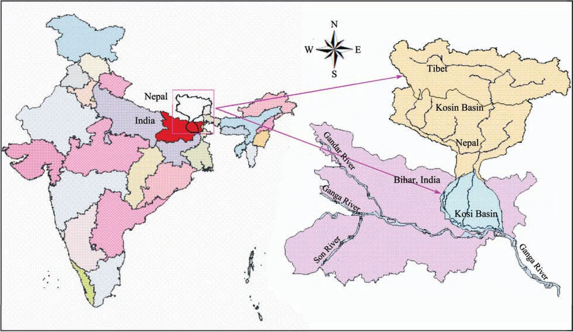
Figure 1 Index map of Kosi River Basin in India, Nepal and Tibet

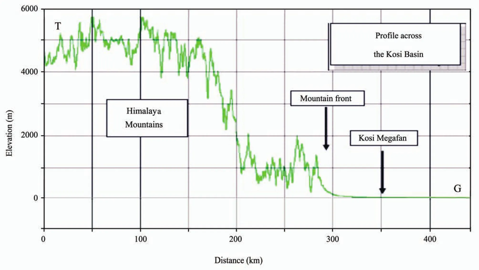
Figure 2 Elevation profile across the Kosi River, T=Tibet, G=Ganga River (Source: Kale, 2008)

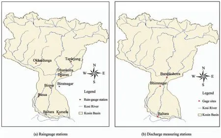
Figure 3 Location of rain-gauge and discharge measuring stations

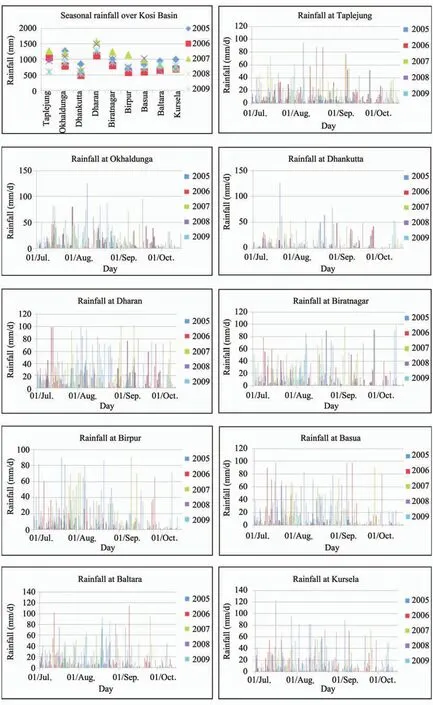
Figure 4 Rainfall time series at different rain-gauge stations

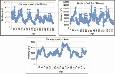
Figure 5 Modified discharge data at different sampling stations

3 Neural network architecture and model development

3.1 The ANN architecture

In the present work, both the Popular Multilayer Perceptron (MLP) network and the Radial Basis Function (RBF)network have been considered for precipitation-runoff modeling. By the simplicity of their architecture and training method, RBF networks are an attractive alternative respective to MLP. At present, RBF and MLP are two models of neural networks with the greatest popularity for pattern recognition tasks. They are a clear example of feed forward neural networks with nonlinear layers (Hutchinsonet al.,1994). These techniques can be used as universal approximation, and are trained in a similar way with the descendent gradient method (Ding and Xiang, 2004). For these kinds of problems, there are always RBFs capable of making a level of accuracy equal to MLP, andvice versa. However, both networks have important differences (Fuet al., 2002).

In this work, variations of soil temperature were monitored.

(1) RBF has a single hidden layer, and MLP can have one or more.

(2) Generally, in MLP all hidden and output nodes have the same neural model. On the other hand, in RBF the hidden and output nodes have different neural models.

(3) The parameters of the activation function for each hidden node in RBF are calculated with the Euclidean distance between the input vector and the prototype vector. Moreover,the parameters of the activation function of each hidden unit in MLP are calculated from the sum of the product between the input vector and the synaptic weights of each unit.

(4) MLP generates a global approximation for the nonlinear association of input-output. Furthermore, RBF networks generate a local approximation for the nonlinear association of input-output.

The MLP architecture of ANN for precipitation-runoff modeling is shown in Figure 6. MLP assumes that the unknown function (precipitation-runoff) is represented by a multilayer feed forward network of sigmoid units.

3.2 Model development

An ANN model withninput neurons (X1, …,Xn),hhidden neurons (W1, …,Wh) andmoutput neurons (Z1, …,Zm) is considered in this study. The function that this model calculates is:

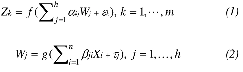
wheregandfare activation functions,i,j, andkare representing input, hidden and output layers respectively,jis the bias for neuronWjandkis the bias for neuronZk,ijis the weight of the connection from neuronXitoWjandjkis the weight of the connection from neuronWjtoZk.

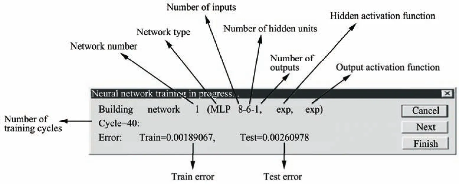
Figure 6 MLP Network used for Kosi Basin, India

The hyperbolic tangent sigmoid function is used in this study as activation function for the hidden nodes. The function can be written as the following:

whereSiis the weighted sum of all incoming information and is also referred to as the input signal:

The major advantage of MLP is that it is less complex than other artificial neural networks such as RBF, and has the same nonlinear input–output mapping capability (Coulibaly and Evora, 2007). The training of MLP involves finding an optimal weight vector for the network. The objective function of the training process is:

whereNis the number of training data pairs,Mis the output node number,Tkpis the desired value of thekthoutput node for input patternp, andZkpis thekthelement of the actual output associated with inputp(Antaret al., 2006).

4 Input data selection and analysis

For the model development, data sets were divided in training, testing and validation components randomly in STASTICA software. The input data used was mean antecedent total daily precipitation {P(t-1), …,P(t-n)}, mean total rainfall of the current day from each rain-gauge {P(t)},and antecedent daily mean discharges from the outlet gauge{Q(t-1), …,Q(t-n)}. Since the time sequence is important,the sequences of input arrangement are in order. The output from the model is the simulated mean daily runoff {Q(t)}.

According to the autocorrelation (ACC) properties and cross correlation (CCC) between daily rainfall and runoff series, different input variables can be used for ANN. In the present work, based on ACC and CCC of rainfall and stream flow time series at different lags, five models, as shown below,were used to investigate the number of antecedent events needed to obtain optimal results for daily runoff forecasting:

(a) Q(t)={P(t)}

(b) Q(t)={Q(t-1)}

(c) Q(t)={P(t),P(t-1)}

(d) Q(t)={Q(t-1),Q(t-2)}

(e) Q(t)={P(t),P(t-1),P(t-2)}

(f) Q(t)={P(t),P(t-1),P(t-2),Q(t-1)}

(g) Q(t)={P(t),P(t-1),P(t-2),Q(t-1),Q(t-2)}

In the first step, the input data for MLP networks were considered. The random order was used for training material and the Levenberg-Marquardt back Propagation algorithm,as the most efficient algorithm (Ramirez-Beltran and Montes, 2002), was used to train the neural network. The training algorithm used was Broyden-Fletcher-Goldfarb-Shanno(BFGS), error function was Sum of Squares (SOS) and the hidden activation for different MLPS was exponential, tank,identity or logistics. No weighting decay was considered in the analysis for hidden units. The training was stopped at 1,000 epochs. The learning rate was set from 0.7 to 0.1 and the learning rule is momentum. Each MLP network contained seven hidden units positioned in each hidden layer.

5 Performance evaluation

The performance of hydrologic models is usually evaluated by the comparison of desired and model predicted values. This comparison can be done by graphical or numerical methods. Global statistics (Root Mean Squared Error, and Correlation Coefficients (Legates and McCabe, 1999; Harmel and Smith, 2007)) are usually used for model calibration or comparison of different models.

It is noted that Unalet al. (2004) validated simulation models by using statistical characteristics such as average,standard deviation, skewness coefficient, autocorrelation coefficient, maximum and minimum values, and performance criteria such as relative error, absolute error, fre-quency of success, ranges of relative and absolute errors. Liuet al. (2003) validated the results of ANN models with root mean square error and determination coefficient. Most recently, Aksoy and Dahamsheh (2009) used a multi-criteria validation of ANN models developed for Jordan by using graphical and numerical measures, including forecasted and observed time series, scatter diagram, residual time series between forecast and observation, mean absolute and relative errors between forecast and observation, dimensionless mean absolute error and dimensionless mean relative error between forecast and observation. Additionally, the following performance measures were adopted: Determination coefficient to quantify the linearity between forecast and observation, mean square error, mean absolute error; andaandb(slope and intercept) in the best fit linear line of the scatter diagram between forecast and observation.

As there is no single definite evaluation test, it is important to apply a multi-criteria assessment of ANN skill(Dawsonet al., 2002; Kumaret al., 2005). These statistics are summarized in a recent paper by Dawsonet al. (2007)and could be calculated automatically on the Hydro test website available at www.hydrotest.org.uk. In the present work 17 criteria of global statistics were used, which are absolute maximum error, coefficient of efficiency, index of agreement, mean absolute error, mean absolute relative error or relative mean error, medium absolute percentage error,mean error, mean relative error, mean squared relative error,peak difference, error in peak, coefficient of persistence,correlation of determination, relative absolute error, fourth root mean quadrupled error, root mean squared error, and relative volume error. The reader is referred to Dawsonet al.(2007) for the mathematical formulation of these criteria. The description of two criteria, used in the present work is RMSE and correlation coefficient. They are discussed below.

To verify the developed ANN models, global statistics such as Root Mean Square Error (RMSE), and coefficient of correlation were used. Furthermore, the non-parametric test for equality of the mean, variance and probability distribution of observed and simulated runoff was used to validate rainfall-runoff models and to compare them with global statistics.

RMSE (also called the Root Mean Square Deviation,RMSD) is a frequently used measure of the difference between values predicted by a model and values actually observed from the environment that is being modeled. These individual differences are also called residuals, and RMSE serves to aggregate them into a single measure of predictive power. The RMSE of a model prediction with respect to the estimated variableXmodelis defined as the square root of the mean squared error:

whereXobsis observed values andXmodelis modeled values at time/placei.

Correlation—often measured as a correlation coefficient—indicates the strength and direction of a linear relationship between two variables (for example model output and observed values). A number of different coefficients are used for different situations. The best known is the Pearson Product Moment Correlation Coefficient (PPMCC) (also called Pearson Correlation Coefficient (PCC) or the Sample Correlation Coefficient (SCC)), which is obtained by dividing the covariance of the two variables by the product of their standard deviations. If we have a seriesnobservations andnmodel values, then PPMCC can be used to estimate the correlation between model and predicted values.

The correlation is +1 in the case of a perfect increasing linear relationship, and -1 in case of a decreasing linear relationship, and the values in between indicates the degree of linear relationship between for example model and observations. A correlation coefficient of 0 means there is no linear relationship between the variables.

The square of the Pearson correlation coefficient (r2),known as the coefficient of determination, describes how much of the variance between the two variables is described by the linear fit.

6 Results and discussion

Using observed precipitation data of all the nine stations,mean daily precipitation was computed using the Thiessen polygon method (Figure 7), considering weighted mean precipitation over an area under each rain gauge station. The following Thiessen formula was used to compute rainfall distribution:

where= spatial average of precipitation,Ai= area of the part of the sub-catchment belongs to the rain gaugei,Pi=rain gauge precipitation value at rain gaugei,n= total number of rain gauges,A= total area of the sub-catchment.

Rainfall data was tested for auto-correlation and cross-correlation to assess the intra/inter-station precipitation data correlation prior to their use as input in the ANN models. A similar approach was also used for the analysis of discharge data. Different combinations of rainfall data and/or discharge data were used in different MLP and RBF architectures of ANN for modeling precipitation-runoff relationships of the Kosi River Basin at locations Barahkshetra,Bhimnagar and Baltara. Figure 8 illustrates training and validation results at three discharge measuring locations of the Kosi River Basin using the RBF algorithm. The results obtained are very poor and do not show strong RMSE and correlation coefficient values.

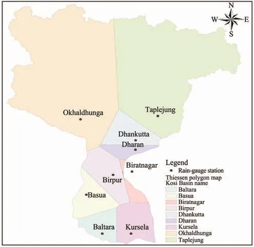
Figure 7 Thiessen Polygon Map for Kosi Basin

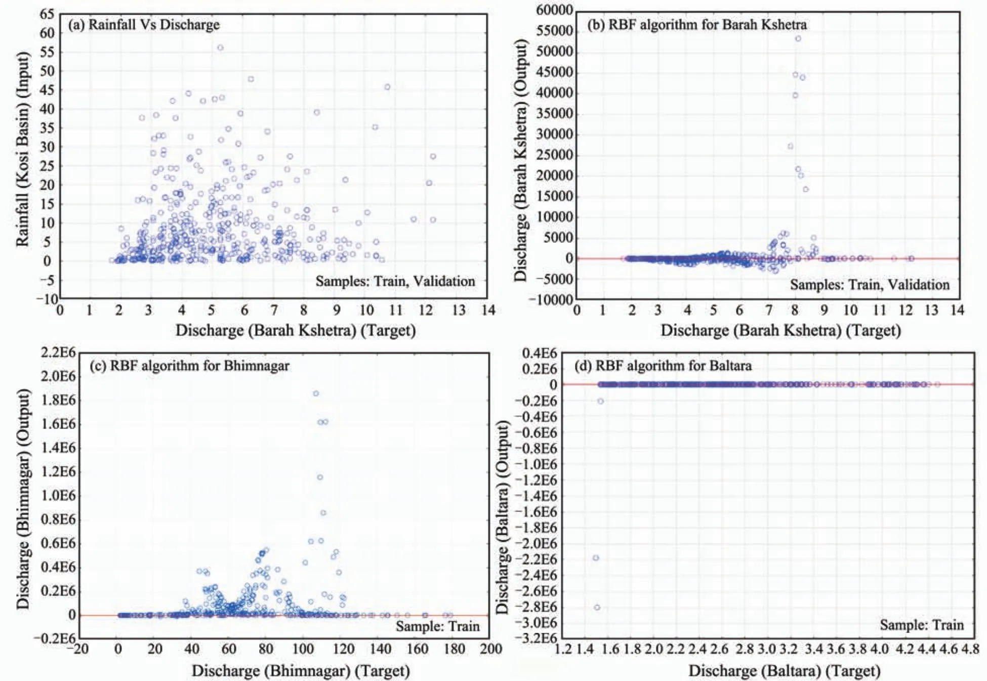
Figure 8 ANN modeling using RBF algorithm

Further, MLP algorithms with different hidden layers were used for their applicability to predict discharge at Barahkshetra, Bhimnagar and Baltara and it is found that MLP with hidden layer three provides best and optimum results with high correlation coefficient (0.97) and less RMSE values (0.01) (Figure 9).

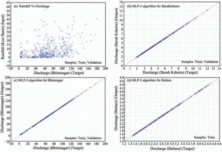
Figure 9 ANN modeling using MLP algorithm

Although the above error statistics provide relevant information on the overall performance of the models, they do not provide specific information about model performances at high or low flows, which are of critical importance in flood or low flow context. The box-plot and probability plot of observed and computed flows were carried out. The probability plot of observed and simulated stream flow was fitted by Blom’s method (Blom, 1958), which is based on the fractional rank of the observation. The parameters of the probability function were estimated by the maximum likelihood method. These tests are useful for visual comparison of the upper or lower tail of the distribution of observed and estimated stream flow. The box-plots of estimated stream flow for MLP-3 at all stations are illustrated in Figure 10.From box-plots, it is clear that the MLP-3 network matched the observed stream flow, especially for higher flows. The probability plots for the MLP-3 network reveal that the distribution of MLP-3 estimated stream flow data are similar for a normal distribution (Figure 11). Furthermore, expected and normal cumulative probability plots have been made with 95% confidence limits (Figure 12). It is observed that MLP with hidden layer three provides the best results.

Figure 10 Box-plots of the discharge data of stations

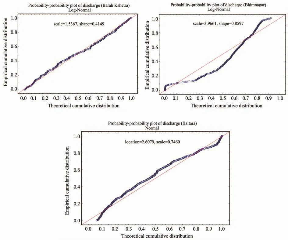
Figure 11 Probability-plots of the discharge data of stations

Figure 12 Expected and observed CDF with 95% confidence limit

7 Conclusion and summary

In the Himalayan regions, artificial neural networks are found to be a powerful tool for modeling nonlinear relationships in rainfall-runoff relationships. The multi-layer perceptron with four hidden layers was selected as the best neural network based on global statistics. However, MLP with different hidden layers was also found to be in good agreement with observed values.

The validation phase of the neural network modeling plays an important role in the efficiency testing of the modeling. Global statistics are common methods used in this phase. However, the findings reported in this paper show that global statistics broadly reflect the accuracy of the model but are insufficient indicators of the best ANN. This is because they do not capture the mean, standard deviation and probability distribution of the observed stream-flow.

Thus, for flood or low flow simulation or forecasting, it is important to check the accuracy of the ANN output separately using box-plots or probability plots. In the present case MLP-3 reproduces probability distribution (normal)and stream flow statistics. This study also shows the advantage of the application of empirical, physical or conceptual models, together with ANN because some of these models may give better results with more simple modeling procedure than ANNs.

The authors would like to express many thanks to National Institute of Technology, Rourkela for providing all facilities during data collection to carry out this study.

Aksoy H, Dahamsheh A, 2009. Artificial neural network models for forecasting monthly precipitation in Jordan., Stoch. Environ. Res. Risk Assess., doi: 10.1007/s00477-008-0267-x (in press and online available).

Antar MA, Elassiouti I, Allam MN, 2006. Rainfall-runoff modeling using artificial neural networks technique: a Blue Nile catchment case study.Hydrol. Proc., 20: 1201–1216.

Blom G, 1958. Statistical estimates and transformed beta variables. John Wiley and Sons, NY, USA, pp. 174.

Coulibaly P, Evora ND, 2007. Comparison of neural network methods for infilling missing daily weather records. J. Hydrol., 341: 27–41.

Dawson CW, Abrahart RJ, See LM, 2007. Hydrotest: A web-based toolbox of evaluation metrics for the standardized assessment of hydrological forecasts. Environ. Model. Softw., 22: 1034–1052.

Dawson CW, Wilby R, 1998. An artificial neural network approach for rainfall-runoff modeling. Hydrol. Sci. J., 43: 47–66.

Dawson CW, Wilby RL, Chen Y, 2002. Evaluation of artificial neural network techniques for flow forecasting in River Yangtze, China. Hydrol.Earth Syst. Sci., 6: 619–626, http://www.hydrol-earth-syst-sci.net/6/619.

Ding SQ, Xiang C, 2004. From multilayer perceptrons to radial basis function networks: a comparative study. IEEE. Conference on Cybernetics and Intelligent Systems, Vol. 1, Singapore, 1–3 December, pp. 69–74.

Elshorbagy A, Simonovic SP, Panu US, 2000. Performance Evaluation of Artificial Neural Networks for Runoff Prediction. Journal of Hydrologic Engineering, 5(4): 424–427.

Fu X, Wang L, Chua KS, Chu F, 2002. Training RBF neural networks on unbalanced data. IX International Conference on Neural Information Processing (ICONIP’02), Singapore, pp. 1016–1020.

Garcia-Bartual R, 2002. Short Term River Flood Forecasting with Neural Networks. Universidad Politecnica de Valencia, Spain, pp. 160–165.

Gautam MR, Watanabe K, Saegusa H, 2000. Runoff Analysis in Humid Forest Catchment with Artificial Neural Networks. Journal of Hydrology, 235:117–136.

Harmel RD, Smith PK, 2007. Consideration of measurement uncertainty in the evaluation of goodness-of-fit in hydrologic and water quality modeling. J. Hydrol., 337: 326–336.

Harpham C, Dawson CW, 2005. The effect of different basis functions on a radial basis function network for time series prediction: A comparative study. Neurocomputing, 69: 2161–2170.

Harun S, Kassim AH, Van TN, 1996. Inflow Estimation with Neural Networks.10thCongress of the Asia and Pacific Division of the International Association for Hydraulic Research, pp. 150–155.

Hsu K, Gupta HV, Sorooshian S, 1995. Artificial neural network modeling of the rainfall-runoff process. Water Resour. Res., 31(10): 2517–2530.

Hutchinson JM, Lo A, Poggio T, 1994. A Nonparametric Approach to Pricing and Hedging Derivates Securities Via Learning Networks. Technical Report, Artificial Intelligence Laboratory and Center for Biological and Computational Learning, MIT, Memo 1471. No. (92).

Imrie CE, Durucan S, Korre A, 2000. River Flow Prediction Using Artificial Neural Networks: Generalization Beyond the Calibration Range. Journal of Hydrology, 233: 138–153.

Kale VS, 2008. Himalayan Catastrophe that Engulfed North Bihar. Journal Geological Society of India, 7: 713–719.

Kumar ARS, Sudheer KP, Jain SK, Agarwal PK, 2005. Rainfall-runoff modeling using artificial neural networks: comparison of network types., Hydrol. Proc., 19: 1277–1291.

Legates DR, McCabe Jr GJ, 1999. Evaluating the use of "goodness-of-fit"measures in hydrologic and hydroclimatic model validation. Water Resour. Res., 35(1): 233–241.

Liu J, Savenije HHG, Xu J, 2003. Forecast of water demand in Weinan City in China using artificial neural networks. Phys. Chem. Earth, 28(4–5):219–224.

Ramirez-Beltran N, Montes JA, 2002. Neural networks to model dynamic systems with time delays. IIET, 34: 313–327.

Tokar AS, Markus M, 2000. Precipitation-runoff using artificial neural networks and conceptual models. J. Hydrol. Eng., 5: 156–161.

Unal NE, Aksoy H, Akar T, 2004. Annual and monthly rainfall data generation schemes. Stoch. Environ. Res. Risk Assess., 18: 245–257.

Zhang B, Govindaraju RS, 2003. Geomorphology-based artificial neural networks for estimation of direct runoff over watersheds. J. Hydrol., 273:18–34.