On Implementing a Practical Algorithm to Generate Fatigue Loading History or Spectrum from Short Time Measurement

LI Shan-shan,HUANG Zhi-bo,CUI Wei-cheng,

(1.State Key Lab of Ocean Engineering,Shanghai Jiao Tong University,Shanghai 200030,China;2.China Ship Scientific Research Center,Wuxi 214082,China)

On Implementing a Practical Algorithm to Generate Fatigue Loading History or Spectrum from Short Time Measurement

LI Shan-shan1,HUANG Zhi-bo2,CUI Wei-cheng1,2

(1.State Key Lab of Ocean Engineering,Shanghai Jiao Tong University,Shanghai 200030,China;2.China Ship Scientific Research Center,Wuxi 214082,China)

Fatigue life prediction requires the information of fatigue loading history or spectrum over the whole design life.However,in many cases,the measured or simulated load history only includes a very short time compared to the entire design life.How to extrapolate the measured loads to longer time and how to count the information for every cycle are two important problems to be solved in fatigue analysis.In this paper,a method to extrapolate the measured loads to longer time is introduced together with the rainflow cycle counting method.Both methods have been implemented into computer programs.An example calculation is given to show the process.Problems on how to use these two methods to determine the design load are also pointed out.

load history;rainflow filter;load extrapolation;load spectrum;rainflow cycle;counting

Biography：LI Shan-shan(1985-),female,Ph.D.student of Shanghai Jiao Tong University;

HUANG Zhi-bo(1984-),male,engineer of CSSRC.

1 Introduction

Fatigue is defined as a process of cycle by cycle accumulation of damage in a material undergoing fluctuating stresses and strains[1].A significant feature of fatigue is that the load is not large enough to cause immediate failure.Instead,failure occurs after a certain number of load fluctuations have been experienced,i.e.after the accumulated damage has reached a critical level.For marine structures such as ships and offshore platforms they are subjected to this type of cyclic loading,so fatigue is one of the most significant failure modes[2-4].Accurate prediction of the fatigue life of marine structures under service loading is very important for both safe and economic design and operation.

It is well-known that there are two types of fatigue life prediction methods[5].One is the cumulative fatigue damage(CFD)analysis where fatigue loading is expressed as a spectrum.The other is the fatigue crack propagation(FCP)analysis where fatigue loading is expressed as a time history.In this paper we distinguish the fatigue load history with the fatigue load spectrum while many other authors may not make this distinguish,e.g.,Schijve[6].When we say a fatigue load history,it means a time-domain destinction,e.g.P(t).When we say a fatigue spectrum,it means a frequency-domain destinction,e.g.Weibull distribution.The fatigue load history is used in fatigue crack propagation process while the fatigue load spectrum is used in cumulative fatigue damage calculation.

In fatigue life prediction of a structure,both the fatigue loading and fatigue strength are essential parameters.Hence,in order to obtain a proper fatigue design,it is crucial to consider real environmental loads.However,in many cases,the measured or simulated load history only covers a very short time,compared to the entire design life.Therefore,how to extrapolate the measured or calculated short term loads to longer time needs to be solved.The simplest method is to repeat one observed load block until the design life.This has the drawback that only the cycles in the measured signal will appear in the extrapolation,even though other cycles are also possible.In order to allow more extreme loads than the observed ones,statistical theories have to be employed.In Ref.[7],a statistical method is used that was proposed by Dressler et al.[8]where the rainflow matrix is extrapolated using kernel smoothing.An extrapolation method based on statistical extreme value theory[9]in combination with kernel smoothing is presented in Ref.[10].

In 2006,Johannesson[11]proposed an extrapolation method which can be applied to any signal and be used for any purpose.This method is implemented to study its performances and feasibility to be used for marine structures.

For fatigue life analysis,the load time history needs to be converted into cycle sequence or load spectrum.This can be done by choosing a suitable counting method.It is a common consensus that the rainflow cycle counting is the best[6,12].

In this paper,a practical method for extrapolation of a measured time signal to a longer time period,based on statistical extreme value theory is first introduced.Then the method of rainflow cycle counting is introduced.Both methods have been implemented into computer programs.In order to demonstrate the application,the measurements of longitudinal strain in a deck position of a surface ship for 15 minutes[13]are used for extrapolation and rainflow cycle counting.Finally,issues to determine the design fatigue loading using the measured short history are pointed out for further study.

2 Generating longer loading history from short time measurement

2.1 Method for extrapolation of a load history

The methodology introduced here is updated from Ref.[11].The main idea of this method is to repeat the measured load block,but modify the highest maxima and lowest minima in each block.The random regeneration of each block is based on statistical extreme value theory.An example showing the principle of the method is shown in Fig.1,where three repetitions of a measured block are compared to three extrapolated blocks.

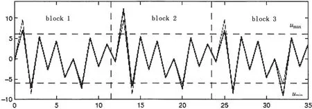
Fig.1 Three repetitions of a measured block(black),compared to three extrapolated blocks(grey).The horizontal dashed lines represent the threshold levels,umin=-6 and umax=6,where the extrapolation starts(Ref.[11]).

The theoretical basis for the method is the so-called Peak Over Threshold(POT)technique in statistical extreme value theory,see Ref.[14].Only the extreme excesses over a high level u is modeled,i.e.the height of the excursions above u,see Fig.2.If we fix a high load level and study the excesses over this level,then under certain conditions these excesses approximately follow an exponential distribution for high enough threshold levels u.We then have the approximation for the excess Z=Max-u∈Exp(m),with cumulative distribution function

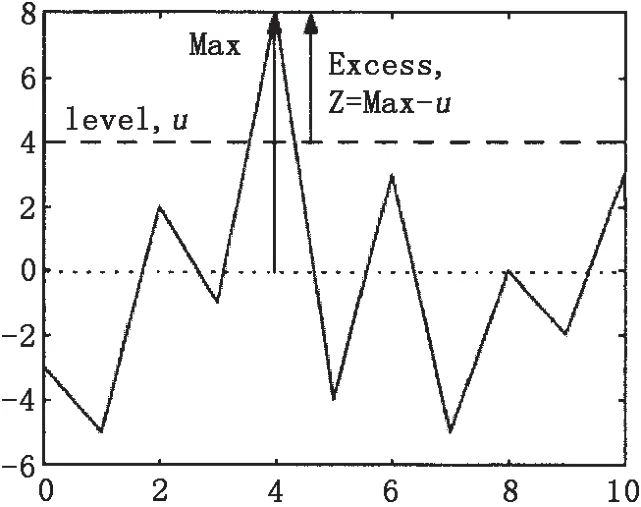
Fig.2 Definition of excess over a threshold u(Ref.[11])

The estimation of the parameter in the exponential distribution is the sample mean of the excesses z1,…,zN

The family of possible distributions for excesses in extreme value theory is the Generalized Pareto Distribution(GPD),

where the shape parameter-∞＜ξ＜∞ and the scale parameter σ＞0.when ξ＜0,the GPD has an upper endpoint,0＜z＜-σ/ξ,while for ξ≥0,z＞0.The special case of ξ=0 is the exponential distribution.The estimation of the parameters in the GPD is known to be problematic,often giving large systematic errors,especially for small sample sizes.Care should be taken for the selection of moment method or maximum likelihood.Details on the maximum likelihood estimation can be found in Refs.[14,27],methods based on moments are discussed in Ref.[28]

Mathematically the extreme value approximations are formulated as asymptotic results.For a random process｛X(t):t∈[0, T]｝satisfying certain mixing conditions,it can be shown that the excesses over a level u(T)converges in distribution to a GPD as T→∞ and n(T)/T→0,where n(T)is the number of excesses over u(T).The parameters of the limiting GPD de-pend on the distributional properties of the process.

As a matter of fact,the exponential distribution of excesses is equivalent to modeling the global maximum as a Gumbel distribution,which works well in many applications.In this section,the model for excesses over a high level will be the exponential distribution,but it is straightforward to replace it by a GPD.

The generation of a k-fold extrapolated signal(sequence of turning points)can be performed in the following steps[11]:

(1)Start with a time signal.

(2)Extract the turning points of the time signal,where the small cycles should be removed by using a rainflow filter.

(3)Choose threshold levels uminand umaxfor the POT extrapolation.The choice of levels is discussed in section 2.2.Extract the excesses under uminand the excesses over umax.

(4)Estimate the mean excesses mminand mmaxunder and over the thresholds uminand umax,respectively.

(5)Generate an extrapolated load block by simulating independent excesses as exponential random numbers.Replace each observed excess under uminby a simulated exponential number with mean mminand each observed excess over umaxby a simulated exponential number with mean mmax.

(6)Repeat step 5 until you have generated k extrapolated load blocks.

(7)The k-fold extrapolated signal is obtained by putting the generated load blocks after each other.

From the k-fold extrapolated load time signal,we can also obtain the k-fold extrapolated load spectrum by applying the rainflow cycle counting algorithm which will be introduced in Section 3.In order to show the method for generating a k-fold extrapolated signal more clearly,a flow chart is given in Fig.3.

2.2 Choice of threshold levels

For the extrapolation,we need to choose the threshold levels where the extrapolation will start(see Fig.2).The choice of proper threshold levels is a difficult problem that demands some judgments.Note that the levels need to be chosen high enough for the extreme value theory to be a reasonable approximation,however also low enough to obtain a sufficient number of exceedances.Hence,it is important to verify that the exponential assumptions are fulfilled for the chosen threshold levels.

A useful diagnostic tool,for assessing the threshold,is the mean excess plot.The estimate of the mean exceedance over the threshold is plotted as a function of the threshold level(see Fig.4).For too low threshold levels,the extreme value approximation is not good enough,giving a systematic error,and for very high levels there is little information giving large scatter,which is seen through the confidence intervals.Hence,a proper level should be a compromise and be chosen somewhere in between in a region where the estimate is stable,i.e.the mean excess plot is approximately horizontal.Unfortunately,the mean excess plots may be hard to interpret,but they are still a valuable tool together with the exponential probability plots.

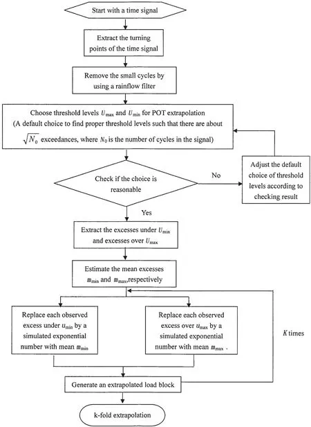
Fig.3 Flow chart of the generation of k-fold extrapolated signal

The choice of proper threshold levels is the most tricky part of the extrapolation.Here one needs to use experience together with the diagnostic tools to ensure that the exponential distribution is a good approximation.A default choice that seems to work well in many cases is to find threshold levels such that there are aboutexceedances,where N0is the number of cycles in the signal.

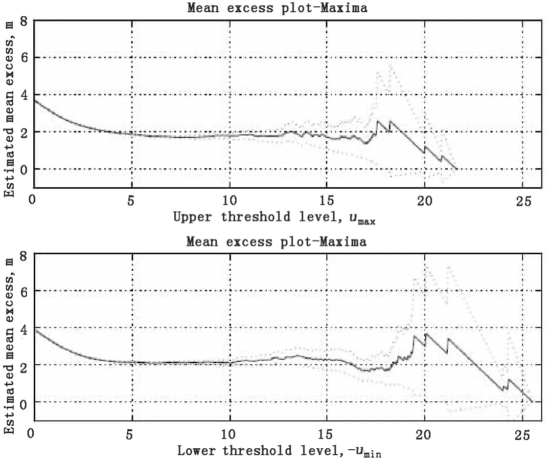
Fig.4 Mean excess plots,i.e.estimate of mean excesses as function of the threshold level,for Norway measurements.The dashed lines represent 95%confidence intervals for the estimate.The threshold level should be chosen in a region where the estimate is stable,i.e.where the plot is approximately horizontal(Ref.[11]).

3 Rain flow cycle counting

Cycle counting is the process of reducing a complex variable amplitude load history into a number of constant amplitude stress excursions,that can be related to available constant amplitude test data.This is a necessary step that needs to be carried out in order to predict fatigue crack growth in components subjected to variable amplitude loading.The method of cycle counting used often depends on the occurrences in the particular sequence that are considered to be significant in terms of fatigue damage[6,12].

The definition of a cycle varies with the method of cycle counting.In fatigue analysis,a cycle is the load variation from the minimum to the maximum and then to the minimum load.At the moment,there is no frequency information contained in any cycle counting method but this can easily be added if three independent quantities are used.Furthermore,some of the counting methods can also give the information of the order of the cycles.Cycle counts can be made for all time histories such as force,stress,strain,torque,acceleration,deflection or other loading parameters of interest.

Cycle counting yields the marginal probability density distribution of the single quantity like amplitude or the joint probability density distribution of the pair such as(maximum,minimum)or(amplitude,mean)or(maximum,range).

Up to now,many different cycle counting methods have been developed such as level crossing counting,range counting and rainflow counting,see Refs.[6,15].One of the most important considerations in cycle counting is that the basis of the counting method needs to be com-patible with the understanding of the relevance of stress fluctuations to the fatigue process.Using this criterion,now it is almost the common consensus that the rainflow cycle counting method is the best cycle counting method[16-17].

The rainflow counting algorithm was first developed by Endo and Matsuiski in 1968[18].Downing and Socie[19]created one of the more widely referenced and utilized rainflow cyclecounting algorithms in 1982,and which was included as one of many cycle-counting algorithms in ASTME 1049-85[16].Rychlik[20]gave a mathematical definition for the rainflow counting method,thus enabling closed-form computations from the statistical properties of the load signal.

In principle,range counting includes counting of all successive load ranges,also small load variations occurring between adjacent larger ranges.It might be thought that small load variations can be disregarded in view of a negligible contribution to fatigue damage.A fundamental counting problem arises if a small load variation occurs between larger peak values.This situation is illustrated in Fig.5.A two-parameter range counting procedure will count the ranges AB,BC and CD,and store this information in a matrix.Now,consider the situation that the intermediate range BC would not occur.Then,the large range AD would be counted only.Traditionally it was thought that fatigue damage is related to load ranges but now it is found that the maximum value is also important[e.g.Refs.21,22].It should be expected that the fatigue damage of the large range AD alone is larger than for the three separate ranges AB,BC and CD.This has led to the so-called rainflow counting method of Endo and Matsuiski[18].The intermediate small load reversal BC is counted as a separate cycle and then removed from the major load range AD.This larger range can then be counted as a separate load range,see Fig.5b.If four successive peak values are indicated by Pi,Pi+1,Pi+2and Pi+3,the rainflow count requirement for counting and removing a small range from a larger range is

If the intermediate small load reversal occurs in a descending load range,see Fig.5c,the requirement is

Fig.5 Intermediate load reversal as part of a larger range[6].

In other words,the peak values of the intermediate small load reversal should be inside the range of the two peak values of the larger range.Successive rainflow counts are indicated in Fig.6.In Fig.6a five rainflow counts can be made.After counting and removing these small cycles,Fig.6b is obtained.In this figure again three rainflow counts can be made,but now of larger ranges.Removing these cycles leads to Fig.6c in which again two still larger load reversals can be counted and removed.In the final residue,Fig.6d,no further counts are possible.The ranges of the residue must be counted separately at the end of the counting procedure.The rainflow count results can be stored in a two-parameter matrix.

The rainflow count procedure has found some support by considering cyclic plasticity.A short load sequence is given in Fig.7a,which leads to counting two intermediate load reversals by the rainflow count method,as indicated in this figure.The corresponding plastic behavior is schematically indicated in Fig.7b,which could be applied to local plasticity at the material surface during the initiation period,or to crack tip plasticity during crack growth.The intermediate load reversals C1 and C2 are causing hysteresis loops inside the major hysteresis of the major cycle between A and B.It is thus assumed that the intermediate plasticity loops do not affect the major loop.This reasoning gives somewhat speculative support to the rainflow counting method.

The rainflow counting method can also be illustrated in Fig.8.The original method was so-called because,if the stress or strain history is presented vertically,the algorithm can be considered analogous to the behaviour of rain flowing from a pagoda style roof.

The rules for this method are as follows[15]:

Let X denote the range under consideration;Y,the previous range adjacent to X;and S the starting point in the history.

(1)Read the next peak or valley.If out of data go to Step(6).

(2)If there are fewer than three points go to Step(1).Form ranges X and Y using the three most recent peaks and troughs that have not been discarded.

Fig.6 Successive rainflow counts[6]

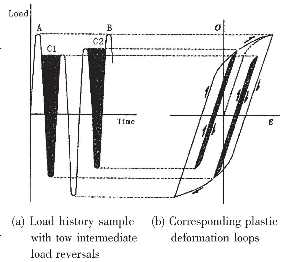
Fig.7 Hysteresis loops associated with rainflow counts[6]

(3)Compare the absolute values of ranges X and Y.

(a)If X＜Y,go to Step(1).

(b)If X≥Y,go to Step(4).

(4)If range Y contains the starting point S,go to Step(5);otherwise,count range Y as one cycle;discard the peak and trough of Y;and go to Step(2).

(5)Count range Y as one-half cycle;discard the first point(peak or trough)in range Y;move the starting point to the second point in range Y;and go to Step(2).

(6)Count each range that has not previously been counted as one half cycle.

These rules may be converted to an algorithm suitable for computation.Commercial program for rainflow cycle counting is also available now,e.g.Durability Rainflow Cycle Counting 2002[23,24].In this paper,a named‘RAINFLOW’code developed by Nieslony[24]is used.It first searches turning points from signals and then carries out rainflow cycle counting according to the algorithm mentioned above.The range and maximum of every cycle can be obtained by an improved edition of this code.

4 A practical example of extrapolation and rainflow cycle counting of a load history

In order to demonstrate the extrapolation and rainflow cycle counting methods introduced above,a full scale test of wave bending moments on a surface ship is used.Fig.9 shows the measurements of the longitudinal strain in a deck position of a surface ship for 15 minutes[13].

Fig.8 The rainflow cycle counting method[15]

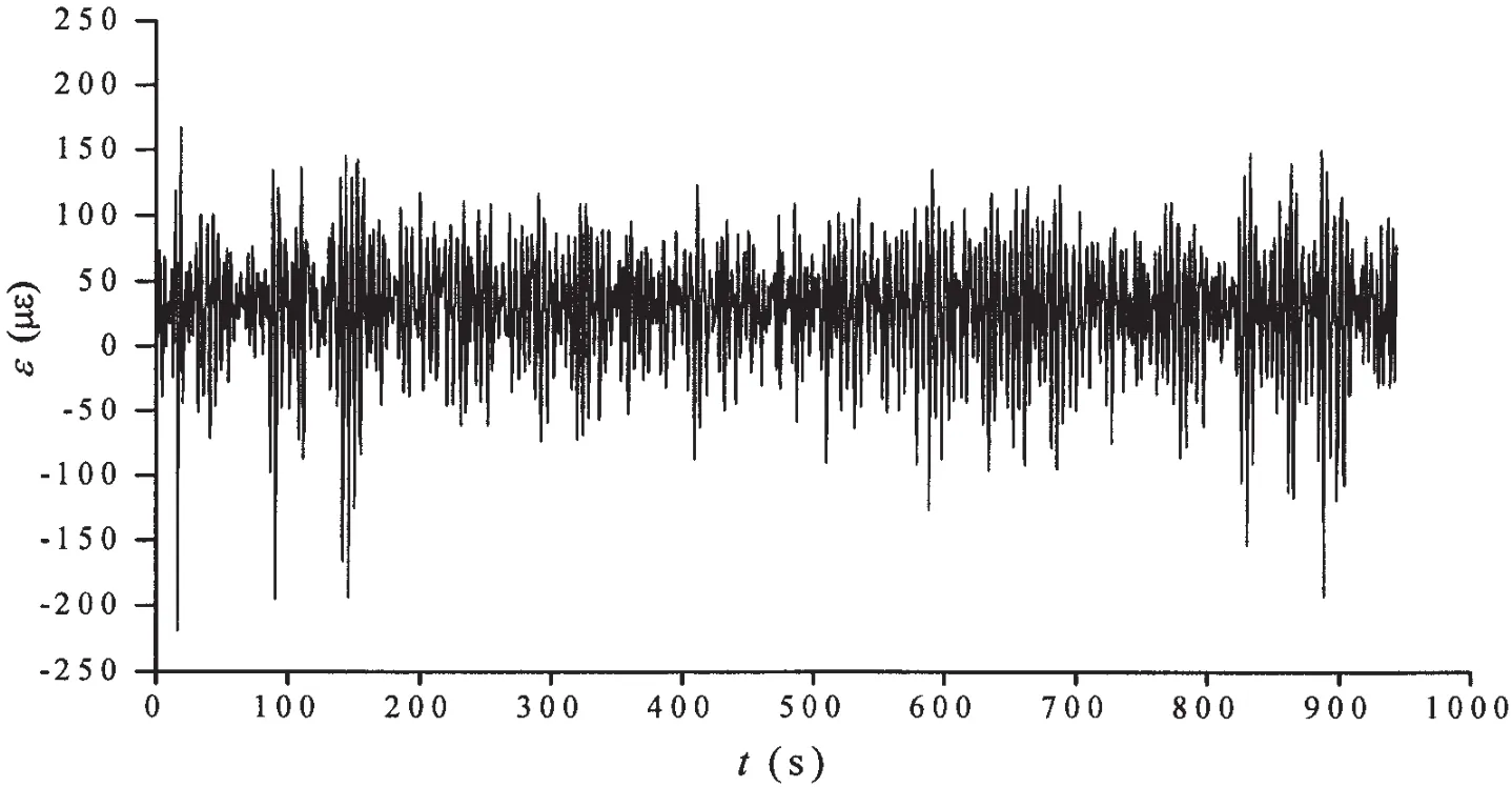
Fig.9 The measured load signals[13]

For this example,we first choose the first three minutes to be extrapolated to a 5 times as a longer time period and compare with the original measurement.First the turning points of the time signal are extracted.Further the signal should be rainflow filtered in order to remove small oscillations that do not contribute to the fatigue damage.It is also advantageous for the POT analysis,since it removes small oscillations during excursions.A default choice for the rainflow filter is to set the threshold range to 5%of the total range of the signal,see Fig.10.Then the threshold levels uminand umaxfor the POT extrapolation are chosen.We choose 121με and-111με as umaxand umin,respectively,see Fig.11.Here we use a default choice to find threshold levels such that there are aboutexceedances,where N0is the number of cycles in the signal.For assessing if the thresholds are proper,we use the mean excess plot method to check it,the result is shown in Fig.12,wherethe chosen threshold levels are in the regions where the estimate is almost stable.With the measured time period increasing,e.g.15 minutes chosen to be extrapolated in this example,the horizontal region in Fig.12 is more clear.The comparison between measured time signal and extrapolated time signal for 15 minutes is shown in Fig.13.

Fig.10 The rainflow filtered load signal for first three minutes

Fig.11 Threshold levels

Fig.12 Mean excess plot

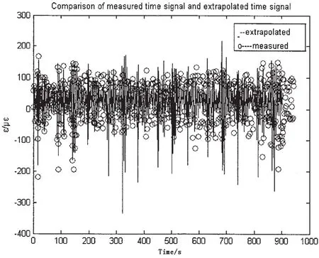
Fig.13 A comparison between measured time signal and extrapolated time signal for 15 minutes

Let us apply the rainflow cycle counting method to the two load-time series shown in Fig.13.For each time series,we will obtain a certain number of complete cycles and some half cycles.For these half cycles,every two half cycles are merged as an equivalent complete cycle and they are put in the end of the series of cycles.For each cycle,we use both maximum and minimum values to represent it.The counted results are shown in Fig.14.

For the counted maximum values and the ranges,they can be plotted as a spectrum.Fig.15a shows a comparison of the load spectra of the 5-fold extrapolations to the 15 minutes of the measured ones for the maximum value of each cycle while Fig.15b shows the range.As is customary,the load spectra are plotted as the cumulative number of cycles larger than a given amplitude as function of the amplitude.We observe that the extrapolation looks reasonable since it agrees well with the observed load spectrum.Further,the load spectra are extrapolated to higher amplitudes,and are smoother compared to the observed ones.These are the properties of the recommended extrapolation method.

Fig.14 Rainflow cycle counted results for two load time signals given in Fig.13(threshold range to 5%of the total range)

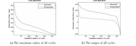
Fig.15 Five-fold extrapolated load spectra compared to the measured load spectra

Now let us take the original measurement of 15 minutes as the source data for extrapolation and to check the effect of folds on the distribution properties.The extrapolation method is based on a random simulation of the high maxima and low minima.Hence,the resulting extrapolated turning points,and hence also the load spectra,will be different from each new simulation.As the number of simulations or the number of folds increases,the load spectra will converge.Fig.16 shows the load spectra for the range of cycles for five different fold numbers:1-fold(original measurement of 15minutes),4-fold(1hour),96-fold(1day).Due to the limit of hard disk,longer extrapolations are not carried out here.

Fig.16 Effect of fold number on the load spectra for the range of cycles

5 Further issues for the determination of design load from the short time measurement

How to construct the design load from limited practical measurements is a very important issue.However,from Fig.16 one may be aware that using different measurement results may result in different design loads if we simply apply the method introduced above.This is certainly not satisfactory from practical application point of view.In order to overcome this deficiency,we suggest to take into account the corresponding wave data information.In order to determine the design load for a specific ship,we first need to provide the time fraction for each sea state,(Si,pi),where i is the sea state number from 0 to 12,0 can be used as the port time,Siis the ith sea state number and piis the time fraction of the ith sea state.Now if we know a short time period of sea state k.We can convert this measurement to different sea states assuming all the responses are in linear range.Then for each sea state,we extrapolate to the corresponding fraction of the design life and count the cycles.Summarizing all the cycles for different sea states,we can derive the load spectra.This load spectrum will be independent of the short time measurements.If the time fraction for each sea state,(Si,pi)has been specified,no matter what sea state is used for the short time measurement,the same design load spectrum will be derived.However,how to construct the time sequence is another challenging problem.This is basically the problem to construct a so-called standardized load history[25-26].This problem will be investigated in the future.

6 Summary and conclusions

Fatigue life prediction requires the information of fatigue loading history or spectrum over the whole design life.There are basically two types of methods to determine the fatigue loads,one is based on calculation and the other is based on experiment.However,in many cases,the measured load history can only include a very short time compared to the entire design life.How to extrapolate the measured loads to longer time and how to count the information for every cycle are two important problems to be solved in fatigue analysis.In this paper,a method to extrapolate the measured loads to longer time has been introduced together with the rainflow cycle counting method.Both methods have been implemented into computer programs.An example calculation is given to illustrate the process.Problems on how to use these two methods to determine the design load are also pointed out.

Acknowledgements

This study was supported by the Innovative Scholars Support Program of Jiangsu Province,Project No.SBK2008004,2008-2010.

[1]Almar-Naess A.Fatigue Handbook[K].Tapir,1985.

[2]Petershagen H.Fatigue problems in ship structures[M].Advances in Marine Structures,Elsevier Applied Science,London,1986:281-304.

[3]Clarke J D.Fatigue crack initiation and propagation in warship hulls[M].Advances in Marine Structures-2,Smith C S and Dow R S,(eds),Elsevier Applied Science,London,1991:42-60.

[4]Liu D,Thayamballi A.Local cracking in ships-causes,consequences,and control[C]//Proceedings:Workshop and Symposium on the Prevention of Fracture in Ship Structure,March 30-31,1995.Washington,D.C.,Marine Board,Committee on Marine Structures,National Research Council,1996.

[5]Cui W C.A state-of-the-art review on fatigue life prediction methods for metal structures[J].J Mar Sci Technol.,2002,7:43-56.

[6]Schijve,Jaap.Fatigue of Structures and Materials[M].Second Edition with CD-Rom.Springer Science+Business Media,B.V.,2009.

[7]Socie D.Modelling expected service usage from short-term loading measurements[J].Int.J Mater.Prod.Technol.,2001,16:295-303.

[8]Dressler K,Gründer B,Hack M,Köttgen V B.Extrapolation of rainflow matrices[R].SAE Technical Paper 960569,1996.

[9]Castillo E.Extreme Value Theory in Engineering[M].Academic Press,San Diego,1988.

[10]Johannesson P,Thomas J J.Extrapolation of rainflow matrices[Z].Extremes 4,2001:241-262.

[11]Johannesson P.Extrapolation of load histories and spectra[J].Fatigue Fract Engng Mater Struct,2006,29:201-207.

[12]Etube L S.Fatigue and fracture mechanics of offshore structures[M].Professional Engineering Publishing Limited,London and Bury St.Edmunds,UK,2001.

[13]Hu Jiajun.The full scale measurement of a surface ship under high sea states[R].Technical Report No.07150,China Ship Scientific Research Center,2007.(in Chinese)

[14]Davison A C,Smith R L.Models for exceedances over high thresholds[J].J Royal Stat.Soc.,Ser.B,1990,52:393-442.

[15]ESDU 95006.Fatigue life estimation under variable amplitude loading using cumulative damage calculations[Z].Issued September 1995 With Amendment A,1995.

[16]ASTM Standard practices for cycle counting in fatigue analysis[K].American Society for Testing and Materials,Philadelphia,PA,USA.E1049-85(Reapproved 1990).

[17]Amzallag C,et al.Standardization of the rainflow counting method for fatigue analysis[J].Int.J of Fatigue,1994,16(4):287-293.

[18]Matsuishi M,Endo T.Fatigue of metals subjected to varying stress[M].Jpn Soc Mech Eng,Fukuoka,Japan,1968.

[19]Downing S D,Socie D F.Simple rainflow counting algorithms[J].Int.J Fatigue,1982,4(1):31-40.

[20]Rychlik I.A new definition of the rainflow cycle counting method[J].Int.J Fatigue,1987,9:119-121.

[21]Vasudevan A K,Sadananda K,Glinka G.Critical parameters for fatigue damage[J].International Journal of Fatigue,2001,23:S39-S53.

[22]Sadananda K,Sarkar S,Kujawski D,Vasudevan A K.A two-parameter analysis of S-N fatigue life using Δσ and σmax[J].International Journal of Fatigue,2009,31:1648-1659.

[23]Rainflow Cycle Counting Software[CP].2002 Release,Durability,Inc.1995-2002.

[24]Nieslony A.Determination of fragments of multiaxial service loading strongly influencing the fatigue of machine components[J].Mechanical Systems and Signal Processing,2009,23(8):2712-2721.

[25]Berger,et al.Betriebsfestigkeit in Germany-an overview[J].International Journal of Fatigue,2002,24:603-625.

[26]Heuler P,Klätschke H.Generation and use of standardised load spectra and load-time histories[J].International Journal of Fatigue,2005,27:974-990.

[27]Grimshaw S D.Computing maximum likelihood estimates of the generalized Pareto distribution[J].Technometrics,1993,35:185-191.

[28]Hosking J R M,Wallis J R.Parameter and quantile estimation of the generalized Pareto distribution[J].Technometrics,1989,29:339-349.

从短期测量数据来生成疲劳载荷的一种实用算法的开发

李珊珊1，黄志博2，崔维成1,2

（1上海交通大学海洋工程国家重点实验室，上海 200030；2中国船舶科学研究中心，江苏 无锡 214082）

疲劳寿命预报需要知道在全设计寿命期内的疲劳载荷时间历程或载荷谱的信息。但是，在很多情况下，实际测量或模拟的载荷时间历程与设计寿命相比只包含很短的一段时间。如何将测量的数据外插到更长的时间段以及如何计数出每周的信息是疲劳分析中必须要解决的两个重要问题。文中的主要目的就是介绍一种将实测载荷外插的方法以及雨流计数法。这两种方法均被编成相应的计算程序。一条水面船的实测数据用作例子来演示计算过程。最后对如何采用这两种方法来构建疲劳设计载荷问题也提出了思路。

载荷历程；雨流过滤器；载荷外插；载荷谱；雨流计数

U662.2

A

李珊珊（1985－），女，上海交通大学海洋工程国家重点实验室，博士研究生；

崔维成（1963-），男，中国船舶科学研究中心研究员，博士生导师。

U662.2

A

1007-7294（2011）03-0286-15

date：2011-01-23

Supported by the Innovative Scholars Support Program of Jiangsu Province(No.SBK 2008004,2008-2010)

王志博（1984-），男，中国船舶科学研究中心工程师；