GPU-accelerated vector-form particle-element method for 3D elastoplastic contact of structures

Wei WANG ,Yanfeng ZHENG ,Jingzhe TANG ,Chao YANG,4 ,Yaozhi LUO,4

1College of Civil Engineering and Architecture,Zhejiang University,Hangzhou 310058,China

2Center for Balance Architecture,Zhejiang University,Hangzhou 310028,China

3Architectural Design and Research Institute of Zhejiang University Co.,Ltd.,Hangzhou 310028,China

4Key Laboratory of Space Structures of Zhejiang Province,Hangzhou 310058,China

Abstract: A graphics processing unit (GPU)-accelerated vector-form particle-element method,i.e.,the finite particle method(FPM),is proposed for 3D elastoplastic contact of structures involving strong nonlinearities and computationally expensive contact calculations.A hexahedral FPM element with reduced integration and anti-hourglass is developed to model structural elastoplastic behaviors.The 3D space containing contact surfaces is decomposed into cubic cells and the contact search is performed between adjacent cells to improve search efficiency.A connected list data structure is used for storing contact particles to facilitate the parallel contact search procedure.The contact constraints are enforced by explicitly applying normal and tangential contact forces to the contact particles.The proposed method is fully accelerated by GPU-based parallel computing.After verification,the performance of the proposed method is compared with the serial finite element code Abaqus/Explicit by testing two large-scale contact examples.The maximum speedup of the proposed method over Abaqus/Explicit is approximately 80 for the overall computation and 340 for contact calculations.Therefore,the proposed method is shown to be effective and efficient.

Key words: Graphics processing unit (GPU);Parallel acceleration;Elastoplastic contact;Contact search;Finite particle method(FPM)

1 Introduction

The numerical modeling of elastoplastic contact of structures is a demanding and challenging task in engineering scenarios (Kang and Kim,2015;Gao et al.,2022).The strong nonlinearities (i.e.,geometrical,material,and contact nonlinearities) involved in elastoplastic contact of structures make it difficult to get accurate solutions (Neto et al.,2017).In addition,the contact calculation processes,especially the contact search and contact constraint enforcement procedures,are usually very time-consuming for large-scale contacts (Wriggers,2006).Therefore,an effective and efficient method is urgently needed to solve the elastoplastic contact of structures.

The finite element method (FEM) is one of the most widely adopted methods for solving the elastoplastic contact of structures.Hallquist et al.(1985) developed the node-to-segment (NTS) contact algorithm in the FEM context,which is simple and reasonably accurate for simulating elastoplastic contacts with large deformation (Hesch and Betsch,2011;Biabanaki et al.,2014).Also,many algorithms have been developed to accelerate the time-consuming contact search procedures,such as the bucket sort algorithm (Benson and Hallquist,1990) and the linear contact search algorithm (Chen et al.,2014).With the rapid development of computer technology,much effort has been put into accelerating contact algorithms using parallel computing techniques (Cai et al.,2015;Cao et al.,2020).However,some procedures of the FEM,such as assembling global stiffness matrices,are inherently difficult to decouple for parallel computing,and lead to undesired computational efficiencies.

In addition to the above numerical methods,a vector-form particle-element method,i.e.,the finite particle method (FPM) (Yu and Luo,2009;Luo and Yang,2014;Yang et al.,2014;Zheng et al.,2021),also has the potential to model elastoplastic contact of structures.The FPM assumes that a structure is discretized into elements and particles.The mechanical properties of the structure are represented by particles instead of elements.The motion equations of particles obey Newton’s second law,and they are solved using explicit time integration techniques.The rigid-body motion of FPM elements can be effectively separated from the total motion of the elements,making the FPM suitable for modeling large-deformation elastoplastic behaviors of structures.In addition,the contact algorithms used in the FEM,e.g.,the NTS algorithm,can be used in the FPM.Furthermore,the FPM is highly parallelizable due to the intrinsically decoupled elemental and particle calculation processes.Therefore,the FPM accelerated by parallel computing techniques is promising as an effective and efficient way of modeling the elastoplastic contact of structures.

There are mainly two kinds of parallel computing strategies: central processing unit (CPU)-based techniques and graphics processing unit (GPU)-based techniques.Specifically,general-purpose computing on GPUs (GPGPU) has been widely used in engineering fields (Hou et al.,2021;Wang SQ et al.,2021) with the development of GPU-oriented application programming interfaces such as NVIDIA compute unified device architecture (CUDA).The GPGPU is more suitable for the parallel acceleration of the FPM than the CPU-based techniques since the elemental and particle calculation procedures can be decoupled and assigned to massive GPU threads.Tang et al.(2020) made the first attempt to develop a universal GPU-based parallel strategy for explicit dynamic analysis using the FPM.Based on this work,the authors proposed a 2D parallel contact algorithm for elastoplastic contacts and achieved a considerable improvement in computational efficiency (Wang W et al.,2021).

In this paper,a GPU-accelerated FPM for 3D elastoplastic contact of structures is proposed.Firstly,a hexahedral element with reduced integration and anti-hourglass is developed to model the 3D elastoplastic behaviors of structures.Subsequently,a 3D parallel contact algorithm is proposed.Specifically,the 3D space containing contact surfaces is decomposed into cubic cells,and the contact search is performed between adjacent cells to improve search efficiency.A connected list data structure is used for storing contact particles to facilitate the parallel contact search procedure.The contact constraints are enforced by explicitly applying contact forces to contact particles.All the computational procedures are designed to be carried out in GPU.The effectiveness and efficiency of the proposed method are verified in four numerical examples.

2 Hexahedral elements in the FPM

This section presents the fundamentals of the hexahedral elements in the FPM.The motion equations of particles and the solutions to the equations are given.Subsequently,the equations of hexahedral elements are described.

2.1 Motion equations

As illustrated in Fig.1,a 3D structure is discretized into particles and hexahedral elements.The motion of each particle in the FPM is governed by the following equation:

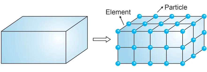
Fig.1 Discretization of a structure

wheremandddenote the mass and displacement of the particle,respectively,Fextis the resultant external force,Fdmpis the damping force,Fcrepresents the contact force (Section 3.3),andFintdenotes the resultant internal force:

whereneis the number of elements containing this particle,idenotes theith element,andis the elemental internal force,which is derived in Section 2.2.The damping forceFdmp=ξdin Eq.(1) is used to account for the mass damping effect,whereξddenotes the mass damping coefficient.

The central difference method is used to derive an explicit solution to Eq.(1):

wheretdenotes the time,Δtdenotes the time step size,c1=(1+ξdΔt/2)-1,andc2=c1(1-ξdΔt/2).

2.2 Elemental internal forces

2.2.1 Fictitious reverse motion

The movement of a hexahedral element within a time step is shown in Fig.2.The reference configuration at timetais denoted byΩa,while the configuration at timetb=ta+Δtis denoted asΩb.The quadrilateral middle surfaces of the element at timestaandtbare denoted byMaandMb,respectively.The four nodes of the middle surfaceMa,denoted asandare midpoints of the edges (1a,5a),(2a,6a),(3a,7a),and (4a,8a),respectively.The total displacement from configurationΩato configurationΩbis denoted as Δd,which is composed of two parts: rigid-body displacement and deformation.The following procedures are performed to eliminate rigid-body displacement of the element.

At first,the configurationΩbis translated to a fictitious configurationΩ′ to make sure that particle 1′ coincides with particle 1a.The fictitious reverse vector is denoted as Δr.

Subsequently,the configurationΩ′ is rotated to fictitious configurationΩ″to ensure that the middle surfaceM″is coplanar with the middle surfaceMa.This out-of-plane rotation is along the axisn′×na,and the rotation angle is

wheren′ andnadenote the normal vectors of the middle surfacesM′ andMa,respectively.

Afterwards,the configurationΩ″is rotated to the fictitious configurationΩ‴to make sure that the inplane rigid-body rotation of the middle surface is eliminated.This in-plane rotation is along the axisn″(the normal vector of the middle surfaceM″),and the rotation angle is

Finally,the deformation vector Δufrom configurationΩato configurationΩ‴is obtained.

2.2.2 Elastoplastic constitutive theory

Once the deformation of a hexahedral element has been obtained,the strain increment of the element Δεcan be calculated by

whereBreflects the strain-displacement relationship.

The equations of the stress increment are related to the material of the element.For elastic materials,the stress increment Δσcan be evaluated as

whereDedenotes the elastic stress-strain relation.In addition,theJ2plasticity model with isotropic hardening is utilized in this study.The yield function is

whereσis the stress,J2denotes the second invariant of the deviatoric stress tensor,andκrepresents the plastic internal variable,which can be regarded as a linear function of the cumulative plastic strain.The detailed formulation of theJ2plasticity model is given in Section S1 of the electronic supplementary materials (ESM).The plastic strain and stress increments in each time step are computed using the radial return algorithm (Simo and Hughes,1998;Borja,2013).

2.2.3 Internal forces

The following equation can be obtained using the principle of virtual work:

Substituting Eq.(6) into the right side of Eq.(9),the elemental internal forcescan be expressed as the following integral form:

The reduced integration in combination with hourglass control techniques (Flanagan and Belytschko,1981) is adopted to solve Eq.(10),and the corresponding element is called FPM-H8R.Note that the elemental internal forces need to be corrected by adding anti-hourglass forces:

3 Parallel contact algorithm

The parallel contact algorithm for 3D structures is described in this section.Section 3.1 discusses the discretization of contact surfaces,Section 3.2 gives the parallel contact search procedures,and Section 3.3 describes the enforcement of contact constraints.

3.1 Discretization of contact surfaces

In a typical contact surface pair,as shown in Fig.3,one contact surface is selected to be the contactor surface and the other to be the target surface.The contact surfaces are discretized using the NTS method.Note that the term “NTS” is referred to as “node-to-face(NTF)” in the following to better describe the 3D contact algorithm in this study.Using the NTF method,the contactor surface is discretized into contactor particles and contactor faces,while the target surface is discretized into target particles and target faces.Note that only quadrilateral contact faces are considered in this study,and they coincide with the faces of hexahedral elements.

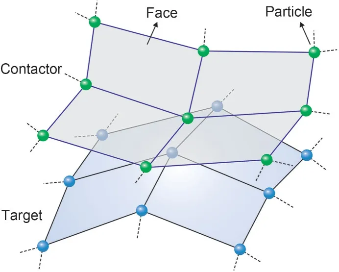
Fig.3 Contact particles and quadrilateral contact faces

3.2 Parallel contact search

3.2.1 Decomposition of 3D space

As illustrated in Fig.4,the potential ranges of motion of all contact particles are:xmin≤x≤xmax,ymin≤y≤ymax,andzmin≤z≤zmax,which can be represented by a bounding box.The box is decomposed into a number of identical cubic cells.The cell sizeLcis proportional to the average characteristic length of all contact faces.

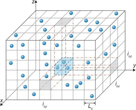
Fig.4 Decomposition of the 3D space containing contact particles

Each contact particleicpin the bounding box is located in a cellic:

whereNxandNydenote the cell counts inxandydirections,respectively.The cell index in each direction is expressed as

where floor(x) represents the largest integer less thanx,and (xcp，ycp，zcp) denotes the coordinate of particleicp.

3.2.2 Connected list data structure

A connected list composed of two arrays is used to store contact particles.This data structure facilitates parallel contact search procedures and also reduces memory requirements in the search procedures.The illustration of the connected list is shown in Fig.5.The first contact particle in each cellicis stored in the arraypHead,while the rest of the contact particles in this cell are linked one by one in the arraypNext.A negative value,such as -1,is used to indicate the termination of the connected list in these two arrays.More details about constructing the connected list data structure can be found in our previous work (Wang W et al.,2021).

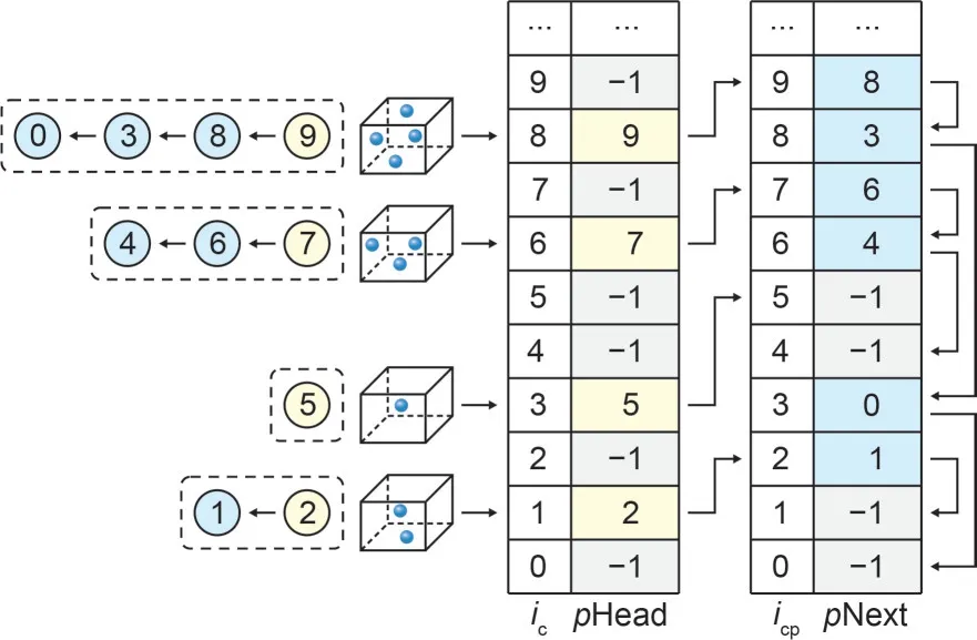
Fig.5 Schematic illustration of the connected list

3.2.3 Search for the closest target particles

Once the connected list data structure has been constructed,the contact search procedure is carried out by searching for the closest target particles for the contactor particles.In this work,only target particles within cellicand the adjacent 26 cells around cellicwill be searched (Zang et al.,2011),which significantly reduces the computational cost of the contact search.The algorithm for the parallel contact search procedures is summarized in Algorithm S1 of the ESM.

3.2.4 Projection onto target faces

After the closest target particles have been found,each contactor particle is then projected onto the target faces.As shown in Fig.6,the contactor particlePcis projected onto target faceSithat is connected to the closest target particlePt,and the projection point ispi.An isoparametric transformation between faceSiand the quadrilateral isoparametric element is built,and the natural coordinate (ξi，ηi) ofpiis obtained.The projection pointpiis insideSionly if the following condition is met:

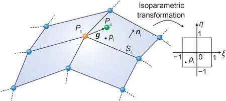
Fig.6 Projection of contact particles onto target faces

The gap vector that points fromPttoPcis denoted byg,and the normal gap is calculated by

wherenidenotes the normal vector ofSi.In a typical contactor particle-target face pair as depicted in Fig.6,the particlePcand the faceSiare assumed to be separated if a positive normal gap (gn≥0) is obtained,and it is not necessary to compute contact forces in this case.By contrast,contact constraints should be enforced on contact particles that show a negative normal gap(gn＜0).

3.3 Enforcement of contact constraints

The enforcement of contact constraints is performed by directly exerting contact forces on contact particles.The contact forces are computed using the equations of the penalty method.

3.3.1 Non-penetration constraint

The normal contact forces are applied to contact particles to ensure that contactor particles do not penetrate into target faces.Using the penalty method,the normal contact force of particlePcis obtained by

wherekn,iis the normal penalty stiffness (Hallquist et al.,1985) of the target faceSi.The expression ofkn,iis given in Section S3 of the ESM.

3.3.2 Friction constraint

The tangential contact forces,i.e.,friction forces,are exerted on contact particles to account for friction between contact surfaces.The friction force of a contactor particle-target face pair is computed based on the smoothed friction model (Benson and Hallquist,1990).Given the friction forceat the previous time step (t-Δt),and the normal contact forceone can compute the friction force at the current time step:

wherekt，irepresents the tangential penalty stiffness,represent the relative displacements of this contactor particle-target face pair at the previous time step and the current time step,respectively.The expression ofkt，iis given in Section S3 of the ESM.

4 Parallel implementation

The proposed method is implemented based on the software developed in our previous studies (Tang et al.,2020;Wang W et al.,2021) using Visual C++and CUDA toolkit.This section focuses on the parallel implementation of the proposed method.

4.1 Flowchart of parallel FPM solvers

The implementation of the proposed method mainly consists of element,contact,and particle solvers.The flowchart of the parallel FPM solvers is given in Fig.S1 of the ESM.At a certain time step,these three solvers are executed sequentially.The computational procedures in the solvers are performed in GPU threads,and the thread counts are listed in Table S1 of the ESM.

4.2 GPU memory optimization

Among all kinds of GPU memories,i.e.,device memories,the global memory has the largest memory space and can be accessed by all GPU threads during their executions.Thus,the global memory is used to store all simulation data in FPM solvers.

The aligned and coalesced memory accesses are required to maximize the global memory bandwidth(Bartezzaghi et al.,2015).To this end,the simulation data in FPM solvers is organized using the storage pattern of SoA (structure of arrays) (Cheng et al.,2014;Lacasta et al.,2014).For example,the device arraypForce is a typical array used to store resultant forces of particles,which can be represented by aNp×3 matrix,whereNpdenotes the number of particles.This array is organized using the SoA memory layout,as shown in Fig.7.The force componentfxis first stored in the array for each particle one by one,followed by the componentsfyandfz.If there is a memory operation that needs to access the componentfx,then the threadst0,t1,t2,… accessf0x,f1x,f2x,… simultaneously.Because the memory addresses off0x,f1x,f2x,… are adjacent to each other,aligned and coalesced memory accesses are achieved.

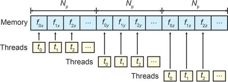
Fig.7 SoA memory layout

5 Numerical examples

This section presents several verification examples and efficiency tests.The hexahedral element FPMH8R is used in FPM,while the linear brick element with reduced integration C3D8R is used in Abaqus/Explicit.The surface-to-surface contact approach and the penalty contact method are used in Abaqus to model contact.

5.1 Verification examples

Two verification examples are investigated to demonstrate the effectiveness of the proposed method.The first example is an elastic contact case,which is given in Section S5 of the ESM.The second example is an elastoplastic case,which is presented in the following.

The “squeezed plastic tube” example (Seitz et al.,2015) is studied.As shown in Fig.8,a cylindrical tube structure is squeezed in the middle by two rigid cylindrical dies.The length,inner radius,and outer radius of the tube are 400,40,and 50 mm,respectively,while those of the dies are 200,45,and 50 mm,respectively.The tube and the rigid die are discretized into 71680 and 1280 hexahedral elements,respectively.

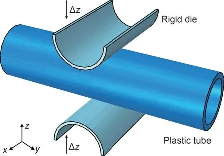
Fig.8 Squeezed plastic tube: geometry

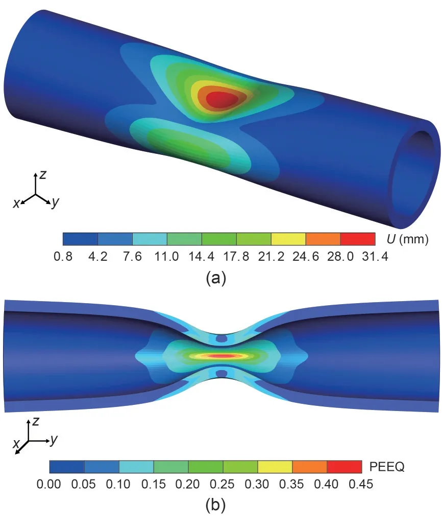
Fig.9 Contour plots of the tube: (a) displacement U;(b) equivalent plastic strain PEEQ

The two cylindrical dies are subjected to prescribed displacements of Δz=30 mm towards each other fromt=0 tot=1 s.Young’s modulus and Poisson’s ratio of the tube are 2069 MPa and 0.29,respectively.The plastic properties are given by the initial yield stress of 4.5 MPa and the isotropic linear plastic modulus of 1.0 MPa.The friction coefficient between all contact surfaces is 0.3.The scaling factorssnandstare set to 0.10 and 0.01,respectively.The mass damping coefficient is set to 10.0.

The displacement contour and equivalent plastic strain contour are presented in Figs.9a and 9b,respectively.It can be found that the plastic regions mainly appear near the middle position of the tube along the axial direction.The time history of total contact forces subjected by the upper die is depicted in Fig.10.The result obtained by FPM is compared with that obtained by Abaqus as well as that in the literature (Seitz et al.,2015) using the semi-smooth Newton method.The above results are in good agreement,indicating the feasibility of the proposed method in modeling elastoplastic frictional contact of structures undergoing large deformation.

Fig.10 Squeezed plastic tube: total contact forces

5.2 Efficiency tests

The efficiency tests of the proposed method are performed on a computer with double precision.The configuration of the computer is given in Section S6 of the ESM.Two large-scale contact examples are tested.A quasi-static elastic contact example is given in Section S7 of the ESM,and a dynamic elastoplastic contact example is given in the following text.Note that the contact face count and the element count have the same order of magnitude in the above two examples,thus the contact calculation time and the total computational time are comparable.These two examples are solved in three types of solvers,i.e.,the parallel FPM solvers running on a GPU,the serial FPM solvers running on a single-core CPU,and Abaqus/Explicit solvers running on the same CPU.It should be pointed out that the parallel FPM solvers and the serial FPM solvers share the same kernel codes.The speedup ratio is introduced to quantify the performance of the parallel implementation (Wang W et al.,2021).

The elastoplastic contact example is adapted from the dynamic elastoplastic contact of a multilayer plate under impact loading (Sharma et al.,2018).As shown in Fig.11,a cylindrical rod strikes the center of a rectangular multilayer plate.The entire boundary of the plate is constrained.The dimension of the plate is 200 mm×200 mm×5 mm.The radius and height of the rod are 10 and 50 mm,respectively.The initial velocity of the rod isv0=5×104mm/s.

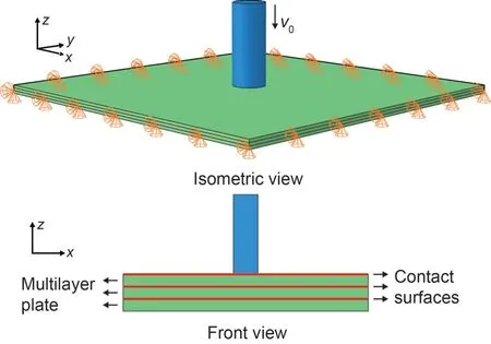
Fig.11 Multilayer plate under impact loading: geometry

The elastic material properties of the plate are given by Young’s modulus of 70 GPa and Poisson’s ratio of 0.3,while the plastic properties are given by the initial yield stress of 285 MPa and the isotropic linear plastic modulus of 900 MPa.Young’s modulus and Poisson’s ratio of the rod are 210 GPa and 0.3,respectively.The densities of the plate and the rod are 2700 and 7850 kg/m3,respectively.The scaling factorsnis set to 1.0.The friction between contact surfaces is ignored.Only a quarter of the model is analyzed due to symmetry.

A three-layer plate is first studied to demonstrate the results.Each layer of the quarter plate is discretized into 2500 hexahedral elements,and the quarter rod is discretized into 240 hexahedral elements.An elastic case and an elastoplastic case are studied,in which the material of the plate is assumed to be elastic and elastoplastic,respectively.The time history of the vertical displacement of the center node on the bottom surface of the cylinder is shown in Fig.12,where the results obtained by FPM and Abaqus are in good agreement.The maximum deformation of the plate in the elastoplastic case is,as expected,greater than that in the elastic case.The deformed configurations of the plate with displacement contours at three instants in the elastoplastic case are presented in Fig.13.The displacement field is continuous at all contact surfaces of the multilayer plate,indicating the effectiveness of the contact algorithm.

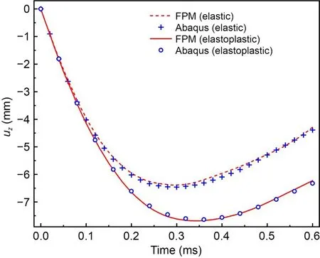
Fig.12 Vertical displacement uz of the cylinder

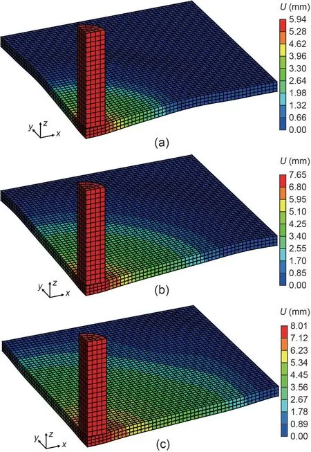
Fig.13 Contour plots of displacement: (a) t=0.15 ms;(b) t=0.25 ms;(c) t=0.35 ms

Multilayer plates with five groups of layer counts are studied to test the efficiency of the parallel FPM solvers in elastoplastic contacts.Each layer has a thickness of 0.25 mm and is discretized into 62500 (250×250×1)hexahedral elements.All cases are solved with a time period of 0.02 ms and a constant time increment of 2×10-5ms.The material of the plate is assumed to be elastoplastic.

The computational times of contact calculation and overall computation are given in Table S4 of the ESM.Specifically,the CPU time consumed by Abaqus contact solver is approximated by Eq.(S5) of the ESM.

The speedups of this example are shown in Fig.14.In respect of the contact calculation,the parallel FPM is approximately 148 times faster than the serial FPM,while 313 times faster than Abaqus.In respect of the overall computation,the above maximum speedups are 132 and 75,respectively.

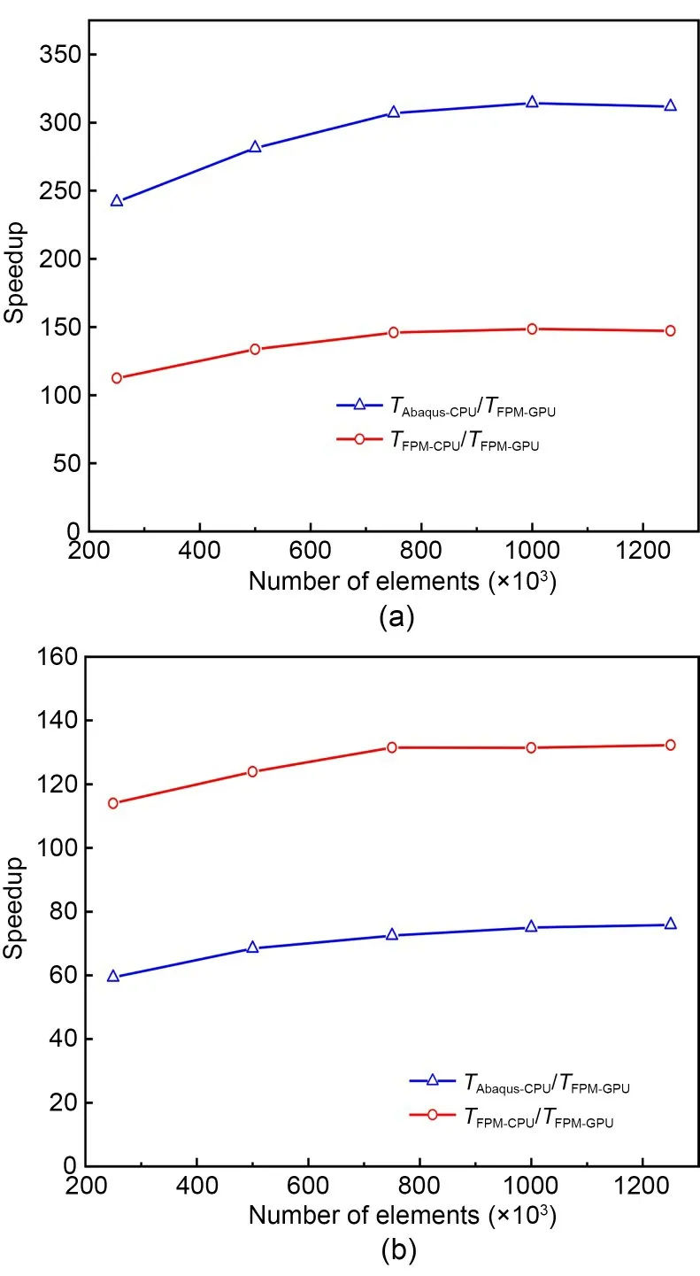
Fig.14 Multilayer plate under impact loading: (a) speedup of contact calculation;(b) speedup of overall computation

Fig.14 also indicates that the GPU is running at full load when the number of elements reaches approximately 0.8-1.2 million,and the improvement of computational efficiency gradually stabilizes.Similar observations can be found in the literature (Dong et al.,2015).One can achieve higher speedups by using GPUs with larger device memory and more CUDA cores.

The proportions of contact calculation in the overall computational time are approximately 75%,20%,and 18% in Abaqus,serial FPM,and parallel FPM,respectively,as shown in Fig.15.Therefore,the parallel FPM solvers are proved to be efficient in elastoplastic contacts.

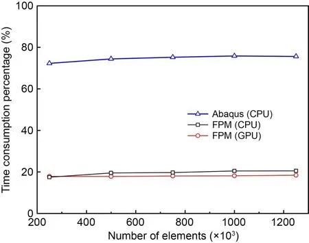
Fig.15 Multilayer plate under impact loading: proportion of contact calculation time

6 Conclusions

A GPU-accelerated FPM is proposed for modeling the 3D elastoplastic contact of structures.A hexahedral element with reduced integration and antihourglass is developed to model structural elastoplastic behaviors.In addition,a 3D contact algorithm is proposed.The whole computational procedures of the FPM are implemented to be executed on a GPU.Four illustrative examples are investigated to show the effectiveness and efficiency of the proposed method.Several observations can be drawn:

1.Two verification examples that involve elastic and elastoplastic frictional contacts are investigated.The results obtained by FPM are consistent with the reference results.Thus,the proposed method is effective.

2.The efficiency of the GPU-accelerated FPM is investigated by testing two large-scale contact examples and it is shown that the proposed method is efficient in both elastic and elastoplastic large-scale contacts.

3.The GPU-accelerated FPM is approximately 130-140 times faster than the serial one,and 70-80 times faster than Abaqus.Specifically,the GPU-accelerated FPM contact solver is approximately 110-140 times faster than the serial FPM contact solver,and 310-340 times faster than the Abaqus contact solver.

4.The time proportions of the contact calculation in the overall computation are approximately 18%-19% in the GPU-accelerated FPM,and 75%-80% in Abaqus,indicating that the proposed method dramatically decreases the time consumed in contact calculation processes.

In summary,the proposed method is shown to be efficient,while maintaining computational accuracy,and is promising for modeling large-scale contact in structures.In future work,parallel acceleration using multiple GPUs simultaneously could be studied to further improve the computational efficiency.

Acknowledgments

This work is supported by the National Natural Science Foundation of China (Nos.51908492,52008366,and 52238001)and the Zhejiang Provincial Natural Science Foundation of China (Nos.LY21E080022 and LQ21E080019).

Author contributions

Wei WANG conducted the research and wrote the manuscript.Yanfeng ZHENG and Chao YANG helped design the research.Yanfeng ZHENG and Jingzhe TANG revised the manuscript.Yaozhi LUO provided funding and supervision.

Conflict of interest

Wei WANG,Yanfeng ZHENG,Jingzhe TANG,Chao YANG,and Yaozhi LUO declare that they have no conflict of interest.