High-emitter identification for heavy-duty vehicles by temporal optimization LSTM and an adaptive dynamic threshold*#

Zhenyi XU, Renjun WANG,2, Yang CAO,3,4, Yu KANG,3,4

1Institute of Artificial Intelligence, Hefei Comprehensive National Science Center, Hefei 230088, China

2AHU-IAI AI Joint Laboratory, Anhui University, Hefei 230601, China

3Department of Automation, University of Science and Technology of China, Hefei 230027, China

4Institute of Advanced Technology, University of Science and Technology of China, Hefei 230088, China

†E-mail: xuzhenyi@mail.ustc.edu.cn; kangduyu@ustc.edu.cn

Abstract:Heavy-duty diesel vehicles are important sources of urban nitrogen oxides(NOx)in actual applications for environmental compliance, emitting more than 80% of NOx and more than 90% of particulate matter (PM) in total vehicle emissions.The detection and control of heavy-duty diesel emissions are critical for protecting public health.Currently, vehicles on the road must be regularly tested, every six months or once a year, to filter out high-emission mobile sources at vehicle inspection stations.However, it is difficult to effectively screen high-emission vehicles in time with a long interval between annual inspections, and the fixed threshold cannot adapt to the dynamic changes of vehicle driving conditions.An on-board diagnostic device (OBD) is installed inside the vehicle and can record the vehicle’s emission data in real time.In this paper, we propose a temporal optimization long short-term memory(LSTM) and adaptive dynamic threshold approach to identify heavy-duty high-emitters by using OBD data, which can continuously track and record the emission status in real time.First, a temporal optimization LSTM emission prediction model is established to solve the attention bias discrepancy problem on time steps that is caused by the large number of OBD data streams in practice.Then, the concentration prediction error sequence is detected and distinguished from the anomalous emission contexts using flexible criteria, calculated by an adaptive dynamic threshold with changing driving conditions.Finally, a similarity metric strategy for the time series is introduced to correct some pseudo anomalous results.Experiments on three real OBD time-series emission datasets demonstrate that our method can achieve high accuracy anomalous emission identification.

Key words: High-emitter identification; Temporal optimization; On-board diagnostic device (OBD); Dynamic threshold https://doi.org/10.1631/FITEE.2300005 CLC number: U495; TP311.13

1 Introduction

Vehicle exhaust consists of greenhouse gases and toxic pollutants, which lead to increasingly serious problems such as poor air quality and ecological environment damage(Franco et al.,2013).At present,China’s regional atmospheric environmental problems are increasingly prominent, and mobile pollution sources in the form of heavy-duty vehicles have a huge impact on air quality.There are currently about 19.567 million diesel vehicles in China,which account for only 6.3% of motor vehicles, but heavy-duty vehicles emit more than 80%of total vehicle nitrogen oxide(NOx)emissions and more than 90%of particulate matter(PM)(Ministry of Ecology and Environment of the People’s Republic of China,2022).Most of the ambient NO2is formed through oxidation of NO, which originates mainly from vehicle combustion in cities.Consequently, NO2is considered to be an indicator of road traffic.Moreover, in the presence of O3and other strong oxidants, NO2experiences further atmospheric transformations that result in the conversion of NO2to nitric acid and of SO2to sulfuric acid.These newly formed pollutants are important sources of nitrates,sulphates, and organic aerosols that contribute significantly to the total PM10or PM2.5mass (Karimian et al.,2019).Therefore,urban air quality can be effectively improved if these high-emitting vehicles are rapidly identified for repair or deregistration to reduce the source of vehicle pollutants.

Currently, vehicles on the road must be inspected for exhaust emissions at vehicle inspection stations (VISs) every six months or once a year,where the collected tailpipe emission data are analyzed and rated to identify high-emission mobile sources to be regularly tested for their emission status.

The studies on VIS classification criteria fall into two main categories: fixed emission thresholds and flexible emission thresholds.One type of study attempts to identify fixed criteria for screening.For example, Stephens et al.(1996) set the thresholds for CO, HC, and NOxat 4%, 0.3%,and 0.2%respectively,in their high-emission remote sensing detection study.McClintock (2007) fixed the cut-offpoints for pollutants at 3%, 500 ppm(1 ppm=1×10-6), and 2000 ppm for these three pollutants in the state of Michigan, USA.In 2010,emission standards in Colorado were more stringent and limits were set at 0.5%,200 ppm,and 1000 ppm separately (McClintock, 2011).Emission thresholds vary with the conditions of vehicle operation,so it is difficult to obtain a uniform fixed standard.

Another type of research proposes flexible methods for identifying high-emission vehicles.For example, Smit and Bluett (2011) developed a vehicle emission discrimination method by comparing laboratory test results with actual test results to calculate a correction factor for high-emission sources.Pujadas et al.(2017) proposed a statistical criterion based high-emission identification method for a large amount of actual emission data.In several studies(Guo et al.,2006;Zeng et al.,2008;Xie et al.,2019;Li ZR et al.,2021),machine learning and deep learning were applied to the study of high-emission mobile sources.Guo et al.(2006) developed a back propagation neural network (BPNN) model to predict high-emission sources, using attributes such as acceleration, velocity, plume and multiple pollutant gases as input features.Zeng et al.(2008) created an improved and optimized high-emission prediction neural network by combining a genetic algorithm and aK-nearest neighbors(KNN) algorithm to improve the model prediction accuracy.Xie et al.(2019)proposed an algorithm to calculate adaptive cut points based on CO, HC, and NOxconcentration values.An unsupervised clustering algorithm was used to cluster the vehicle data and label the thresholds of high-emission clusters, and the KNN algorithm was used to detect the test set samples.To address the scarcity of high-emission labels, Li ZR et al.(2021)created a weighted limit learning machine model and introduced an active sampling method to solve the emission sample imbalance problem and reduce the identification error of high-emission sources.

However, the above methods are based on the data collected by fixed monitoring devices, reflect only the instantaneous emission conditions of the vehicle, and ignore the dynamic changes in driving conditions over time.In addition, although VISs can provide accurate and repeatable results in the process of periodic inspection, the disadvantages of high cost and time requirements mean that inspections cannot be carried out frequently.Therefore,the time span of two adjacent tests is large, which increases the stochasticity and uncertainty of the test results.

Mobile and convenient emission testing equipment can overcome the shortcomings of fixed testing devices.In recent years,on-board diagnostic devices(OBDs) have been increasingly used for heavy-duty vehicle emission detection, which can continuously track and record vehicle emission condition information (including NOxemission concentration, fuel consumption, and exhaust flow data).So, it is of great significance to identify high-emission sources based on OBD time-series data streams.However,this information is insufficient for research.The existing studies continue the above fixed conservative criteria to achieve screening.For example, Xie et al.(2021)used time-series emission data to make decisions and create early warning of high vehicle emission conditions by artificially setting thresholds.However, because the vehicles run in various operating conditions, the driving conditions of the same vehicle will change continuously with the passage of time.Moreover,there are many vehicles to be identified in the actual scenario.Therefore, it is diffi-cult to set a constant standard over the whole emission sequence.Fig.1 illustrates an example of the limitation for a constant threshold to identify high emissions.

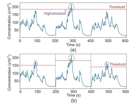
Fig.1 Different thresholds for high-emission identification: (a) constant threshold; (b) dynamic threshold.When the time span of driving conditions is long enough, the constant threshold cannot capture high emissions as accurately as the dynamic threshold

To solve the above problems, a more flexible identification method should be conceived.In this paper, we propose a dynamic threshold approach based on OBD data, which contains real-time vehicle monitoring information such as NOxemission concentration, fuel consumption, and exhaust flow,to achieve adaptive identification of high-emitters.Our main contributions are as follows:

1.Considering the large number of vehicle data streams and the fact that attention bias in historical time can reduce the accuracy of emission prediction for different vehicles,after being inspired by the successful application of the attention mechanism in deep networks (Wu et al., 2018; Li YR et al., 2019;Liu YQ et al., 2020;Xu ZY et al., 2021;Fang et al.,2022), we establish an emission prediction model,long short-term memory (LSTM) based on evolutionary algorithm optimization, which can predict future exhaust emission concentrations more accurately after iterative optimization of the bias weights on time steps.

2.A dynamic anomaly threshold operator is proposed to identify high-emission samples in changing driving conditions, where the decision threshold for high emissions will change adaptively as the driving conditions change with time.

3.An anomaly pruning strategy is introduced that calculates the similarity between normal and abnormal sequences, to correct the possible pseudo anomalous emissions in the identification results and improve the accuracy of high-emission source identification.

In this paper,the proposed method is tested and evaluated with real-time monitoring of OBD data streams of several different motor vehicles in Hefei,China.The results show that our proposed method is more accurate and effective for the identification of high-emission vehicles.

2 Related works

Essentially,the identification of high-emitters is a binary classification problem that includes normal and abnormal emissions.This issue can be transformed into a time-series anomaly detection problem by adding a temporal dimension.The main classical anomaly detection algorithms are solitary forest(isolation forest)(Liu FT et al.,2008),single classification support vector machine (SVM) (Lukashevich et al.,2009),and clustering-based algorithms(Jiang et al., 2001; He et al., 2003; Xu XW et al., 2007).Most of them use statistical features to find outliers.

The research methods for anomaly detection vary with the data.The main anomaly detection research is given in the supplementary materials.For time-series data, the following three main types of anomalies are considered: point,collective,and contextual(Chandola et al.,2009).Point anomalies are single values away from high-density regions,collective anomalies indicate a series of consecutive values that are anomalous, and contextual anomalies represent data with a large difference from the time period before and after values with large differences.We use these features to help explore anomaly analysis methods and to further characterize the anomalous conditions of mobile source emission processes.In the high-emission vehicle identification task, we focus only on the consecutive time periods of abnormal emissions (contextual anomalies), because this appears to be of more practical interest.

Univariate time series represents the data output from a single source linked with the time of the observation.Examples are the current trading price for a stock or share, the electrical signal from a single trace in an electroencephalogram (EEG), total network traffic at a specific time step, or the value produced by a single Internet of Things (IoT) sensor.The structure of the underlying system being monitored is of high importance to the performance of any univariate anomaly detection method.

Continuous temporal data are often available in different application areas,but in the study of mobile source pollution emissions,exhaust gas detection devices are mostly fixed and placed on the driving road.Therefore, these devices can collect only instantaneous data when the vehicle passes by, making it difficult to conduct emission studies over a continuous time period.Based on this fact, researchers prefer to use the spatial and temporal characteristics of exhaust gas detection devices to capture abnormal(high-emission)sources.The experimental data used in our study are derived from OBDs,which can acquire online monitoring data of individual vehicles in real time, breaking the spatial and temporal limitations of fixed detectors and allowing us to conduct studies based on continuous time emission data of vehicles.

3 Preliminaries

In this section,we give some definitions involved in the research work and experimental process, and show the vehicle emission data flow and the way by which the time-series working condition dataset is constructed.

Because actual road types are diverse,the driving conditions of a vehicle can change over time.At the same time, enormous vehicles are being monitored.Thus, it is difficult to use a fixed emission threshold standard for all tested targets.Therefore, we consider high-emission screening based on the actual operating conditions of each vehicle.The definition of the working conditions data stream for a single vehicle derived from the OBD is presented next.

3.1 Single-channel data stream

The dataset used in this study is derived from the OBD carried by the vehicle,and the timing data of a single vehicle are defined as a single-channel data stream.By setting up a single-channel data stream,the independence of different vehicle data information can be ensured, so the OBD data of different vehicles can be separately processed and analyzed by the model.

In addition,maintaining a single model for each channel helps provide finer-grained control of the system.For example, vehicle emission concentration prediction depends on the time-step length,and there is a degree of variation in the attention bias of different vehicles for time steps of the same length.Therefore, processing different vehicle data streams independently can help determine the(approximate)optimal attention weight coefficients and thus improve the prediction accuracy of the model for emission values.

3.2 Time-series condition construction

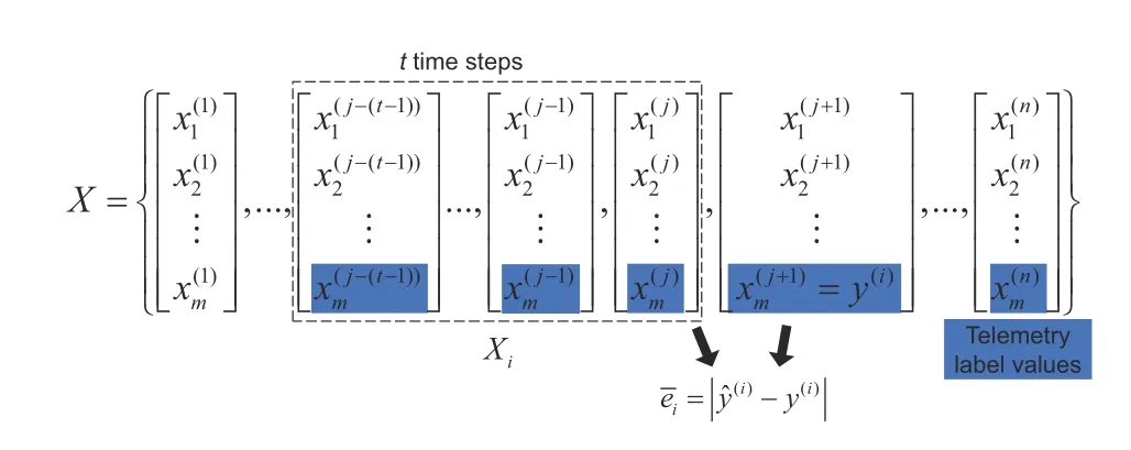
Fig.2 Dataset of the time-series working conditions for an on-board diagnostic device (OBD)

4 Methodology

4.1 Framework

We use a vehicle equipped with an OBD and acquire its real-time emission data online.We track and monitor the exhaust emission status of a single vehicle over a long time series to achieve more accurate high-emission detection than the road network monitoring level.

The single-vehicle high-emission detection problem is transformed into a prediction-based timeseries anomaly detection problem in a practical scenario.First, considering the problem of biased differences in the prediction time steps for various vehicle data streams, an evolutionary algorithm is used to optimize the LSTM time-series prediction model,thus enhancing the prediction accuracy of the model for emission concentrations.Then, a dynamic unsupervised anomaly threshold operator is proposed to help the sliding scan window automatically identify the time periods of abnormal emission concentrations.Finally, a dynamic time warping (DTW)temporal similarity measure strategy is introduced to correct the pseudo anomalies in the identification process.Fig.3 shows the structural framework of this method.

4.2 TSAO-LSTM

In this subsection, we describe in detail the stages of the unsupervised anomaly detection method for high-emission vehicles.The method first uses evolutionary algorithms to develop an optimized LSTM model to learn normal time-series condition data streams to predict vehicle emission concentrations for future time periods.A new unsupervised anomaly threshold operator is then used to evaluate multiple different time-series data streams and to determine whether the resulting prediction errors are representative of vehicle ultra-high-emission tailpipes.Finally, a strategy to correct pseudo anomalies is introduced which can help improve the correctness rate.

LSTM is an excellent time-series prediction model, and its flexible memory capability for historical periods of different lengths can help better predict target values.However, it does not pay enough attention to the time step dependencies, so it is difficult to perfectly apply it to vehicle emission prediction tasks.In practical scenarios,various vehicles will have different driving conditions and performance status,which makes it difficult for their corresponding data streams to have the same or similar attention bias over the same historical time step.This directly affects the prediction accuracy of mobile source emission concentrations.

Inspired by the successful application of the attention mechanism to deep networks (Li YR et al.,2019; Liu YQ et al., 2020), we combine the unique characteristics of vehicle OBD data and introduce the evolutionary algorithm to optimize the attention weight layer of the time step before the LSTM layer.Specifically, we establish a network model for a time-step attention optimization based LSTM(TSAO-LSTM) to find the (approximate) optimal solution of attention layer weights.The setX={X1,X2,...,XN}is the prepared attribute data,and the sety={y1,y2,...,yN}contains the corresponding true labels, whereXi(1≤i ≤N) denotes a two-dimensional time-series data with time steptandXi={X1i,X2i,...,Xti}, whose corresponding true value isyi, andXp i ∈Rm(1≤p ≤t) (Fig.2).The working process of TSAO-LSTM is as follows:

1.Initializing populations and individuals: Set the number of individuals in the populationn; each individual hastfragments of coding genes (corresponding to time stept).Each fragment is coded randomly using one-hot coding and the coding length isl.We define the set of attention-weighted gene vectors of the population as

The individual gene vectorWs(s= 1,2,...,n) is denoted as

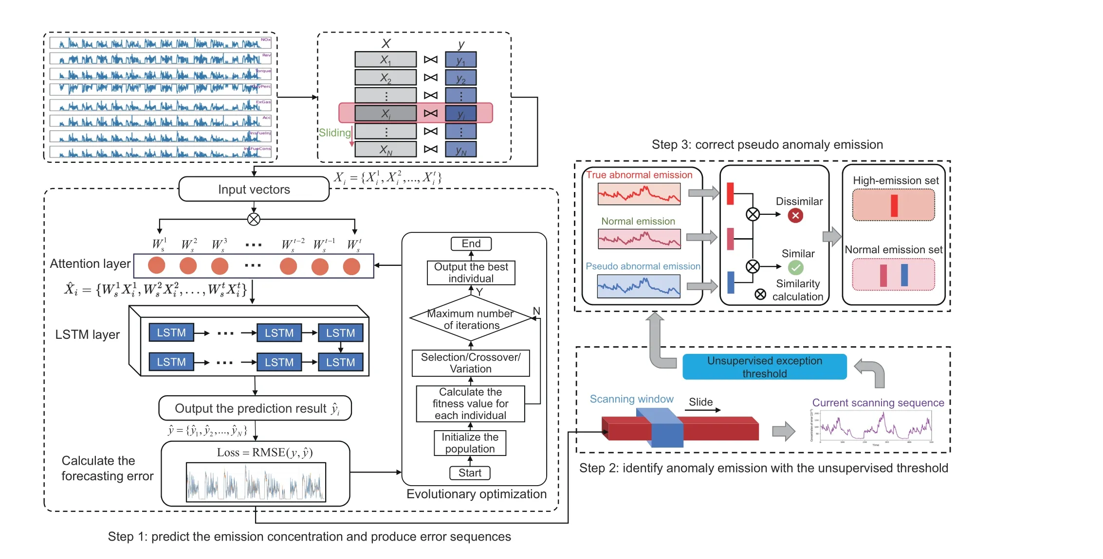
Fig.3 Framework of the research methodology.First, the model for time-step attention optimization based LSTM (TSAO-LSTM) is trained using normal OBD time-series data and predicts the test dataset.The sequence of prediction errors for emission concentration is calculated between the true and predicted values.Then,the scanning window slides on the segmented sequence of prediction errors,and the current unsupervised anomaly emission threshold is calculated accordingly.Specifically,contexts below the threshold are classified as normal emissions and contexts above the threshold are classified as abnormal emissions (including pseudo and true abnormal emissions).Finally, similarity calculations are performed in normal and abnormal emissions.If the similarity is high, the pseudo-abnormal emission is corrected and reclassified to the normal emission set.If the similarity is low, the abnormal emission is classified to the high-emission set

2.Calculating the attention weights and fitness values of the individuals: The one-hot coding value on the individual gene segment is converted into the corresponding decimal value, which will be represented as the attention weight on the time step.For example, for gene segmentWts, its corresponding decimal value is calculated as follows:

whereθdenotes the one-hot gene encoding of lengthl.For ease of explanation, we still use the vectorWs= [W1s,W2s,...,Wts]∈Rtto denote the transformed decimal value vector.After obtaining the weight vector of individuals, the attention mechanism is used to assign different weights to each time step of the input sequenceXito construct a weighted time series ˆXi:

Next, ˆXiis fed into LSTM.The computation process inside the LSTM neuron cell(Yu et al.,2019)is represented as

whereσ(·) represents the sigmoid activation function,Hi-1is the previous hidden state, andHiis the hidden layer output in the current cell.In addition,Iiis the input gate state,Fiis the forget gate state,Ciis the cell state, andOiis the output gate.WI,WF,WC,WOandBI,BF,BC,BOare parameters to learn.Then, the predicted value ofXican be expressed as

Further, the prediction result for this individual on dataX={X1,X2,..,XN}is shown as

We use the loss function result (root mean squared error,RMSE)of the true and predicted values as the fitness value for this individual, and it is expressed as

Finally, the fitness values of thenindividuals of the current population can be obtained.

3.Selection: The population is randomly and equally grouped(each group contains an equal number of individuals), and the best individual with the best fitness value and the two least well-adapted individuals in each group are selected,which ensures a rich diversity of population.

4.Crossover and variation: The excellent individuals selected in step 3 are paired in permutations (2 per pair),and then crossover operations are performed to produce offspring individuals, accompanied by a certain probability of variation.At the same time, to increase the diversity of the current population, two individuals with the worst fitness values will cross over to produce offspring individuals,accompanied by a higher probability of variation.

5.Restructuring a new population: The outstanding parent individuals performing the crossover operation in step (4) and the newly generated off-spring individuals are formed into a new population,and the remaining individuals in the original middle population are eliminated.In particular,the number of individuals of the offspring generated in step 4 is subject to the condition in which the new population and the original population have the same size.

6.Iteration: Steps 2–5 are repeatedptimes,which means that the population has evolved forpiterations.The individual with the best fitness in the last generation of the population is selected as the(approximate)optimal solutionW*of the attention weights to be found.Its optimization effect can be expressed as

whereMdenotes the full parameters in the LSTM layer,and ˆy*denotes the predicted value corresponding to the (approximate)optimal solutionW*.The pseudo code of TSAO-LSTM is given in the supplementary materials.

4.3 Dynamic threshold operator

In practical scenarios, there are often multiple mobile source emission concentration data streams to be detected.In this subsection, we introduce an unsupervised anomaly threshold operator,where the threshold will be calculated based on a dynamically sliding scan window,and a new anomaly threshold is obtained for each slide of the scan window over the sequence.This dynamic scanning approach can help automatically identify anomalies and intervals in the emission concentration sequence.

4.3.1 Representation of the prediction error

At time stept,once the predicted value ˆy(k)forXkin the test set is obtained, the prediction error between it and the true valuey(k)is computed as¯ek=|ˆy(k)-y(k)|(Fig.2).Each ¯ekwill be added to the one-dimensional anomaly vector¯eobtained from the current scan window:

wherehdenotes the number of historical prediction errors used to evaluate the current scan window.

The anomaly vector ¯eis then smoothed using an exponentially weighted moving average(EWMA)(Lucas and Saccucci, 1990), and a new smoothed error vectoreis obtained as follows:

where ˆZt+1is the EWMA value at timet+1, ˆZtandZtare the EWMA and true values at timetrespectively,andθis a weighted constant.

4.3.2 Threshold calculation and abnormality scoring

Normal and abnormal targets are usually distinguished using pre-defined thresholds.However, the threshold itself is a fixed hyperparameter, which requires some manual experience to achieve good and detectable results.However, the time-series data are dynamically changing,and a fixed threshold can limit the fluctuation of the prediction error within the normal range and affect the identification of true anomalies.Therefore, we propose an unsupervised calculation of anomaly thresholds.

The box plot is a well-known method of data analysis and can be used to screen for outliers(Williamson et al.,1989).First,the values in the sequence are arranged in ascending order.Then,some special values are defined: the value located at 1/4 of the sequence is defined as the lower quartile(Q1),the value located at 3/4 of the sequence is defined as the upper quartile (Q3), and the quartile difference value is defined as IQR = Q3- Q1.Finally, the values above Q3+1.5IQR and below Q1-1.5IQR are called outliers.The principle of the box plot is given in the supplementary materials.Inspired by the principle of the box plot,we consider only values above Q3 as possible outliers in our high-emission timing detection work.Furthermore, the threshold valuesαare chosen from the setΦ:

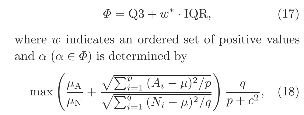
where the anomaly point setA={e*∈e|e*≥α},the normal point setN={e*∈e|e*＜α},μAdenotes the mean value of anomaly points,μNdenotes the mean value of normal points,μdenotes the mean value of the whole sequence,pindicates the number of anomalies,qindicates the number of normal points,andcindicates the number of anomalous contextual sequences consisting of consecutive outliers.

The thresholdαis determined byw*∈w.In addition, values forware closely related to the specific data being processed, and we find that values in the interval [1.5, 2.0] are more suitable for our data.Values forwoutside this range would lead to anomalous misses and false positives.

In summary, we compute the optimal threshold after being inspired by the box plot’s principle,which is initially contained in a set of thresholds and is obtained when it is possible to make expression(18) take the maximum value.This function is suppressed with a multiplicative term at the right end to penalize thresholds that possess a large number of outliers and anomalous sequences.

4.4 Pseudo anomaly correction

Considering the variability and suddenness in actual traffic conditions, vehicle exhaust emission concentration values will increase or decrease sharply within the normal interval within a short time period, while the prediction of the time-series network model often has a certain lag.Therefore, the sudden change values are difficult to predict accurately and lead to spikes of error values (Shipmon et al.,2017).In addition, prediction-based anomaly detection methods depend heavily on the amount of prediction error data (h) contained in the current scan window, which in turn affects the calculation and setting of the unsupervised threshold.In practical scenarios, when the scan window is confronted with large-scale data, it needs to absorb a large amount of historical data, which is costly.The insufficient historical data can lead to anomaly evaluation only in a limited context, which may generate a certain number of pseudo anomalies.

To solve the problem mentioned above, we introduce a pseudo-anomaly correction approach.The pseudo code of the similarity metric algorithm between emission prediction error series using DTW(SMEPES) is given in the supplementary materials.Obviously, there is a huge difference between anomalous and normal sequences.Further, there is a certain difference between the pseudo-anomaly sequence and the normal sequence, but this difference is significantly less than that between the pseudoanomaly and true anomaly.In this context, we introduce a DTW algorithm(Senin, 2008)to measure the degree of difference between different time series,to achieve correction of pseudo anomalies.

For all the abnormal emission concentration sequences initially identified above, we calculate the similarity between them and the normal sequence with the largest emission concentration in the current scan window by the DTW algorithm one by one.The higher the similarity, the smaller the difference; the lower the similarity, the larger the difference.Note that when the length of the anomalous sequences waiting for correction changes, the length of the normal sequences will also change.For example, if the abnormal sequence is known to beA={aLl,...,aL1,aM,aR1,...,aRr}(whereaMdenotes the maximum value inA,aLi(1≤i ≤l)the sequence on the left side ofaMwith lengthl,andaRj(1≤ j ≤ r) the sequence on the right side ofaMwith lengthr), the matching normal sequence isN={nLl,...,nL1,nM,nR1,...,nRr}(wherenMdenotes the maximum value in sequenceN,nLi(1≤i ≤l) the sequence on the left side ofnMwith lengthl, andnRj(1≤j ≤r) the sequence on the right side with lengthr).In conclusion, the relative positions of the maxima in the abnormal and normal sequences are consistent.

5 Experiments and results

5.1 Data and setup

In this study, experiments were conducted on OBD data streams from four different motor vehicles,which came from the urban road monitoring system in Hefei.Details of the OBD dataset are given in the supplementary materials.We used three real vehicle exhaust emission data streams for the evaluation shown in Table 1.

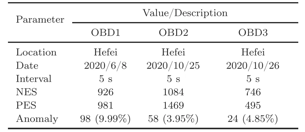
Table 1 OBD experimental data streams

5.2 Model parameters

The hyperparameter settings for the training and prediction phases of TSAO-LSTM model temporal emissions are shown in Table 2.The hyperparameter settings for the attention weighting phase of the evolutionary optimization time step of the TSAOLSTM model are shown in Table 3.

During the sliding window dynamic scanning error sequence, we initialized the sliding window size to 10 and the batch size of a single scan to 20,so the length for the scanned sequence was 200.

Table 2 Base parameters for TSAO-LSTM

Table 3 Evolutionary optimization parameters for TSAO-LSTM

5.3 Baselines

For evaluation purposes, we compared the TSAO-LSTM model to the following baselines:

LSTM:LSTM(Malhotra et al.,2015)is a recurrent neural network (RNN) with flexible historical memory capability that can remember past information,but also selectively forget unimportant information.The model proposed in this paper is improved on this basis according to the actual problem.

GRU: Gated recurrent unit (GRU) (Cho et al.,2014) is a new type of RNN that can be applied to sequences of arbitrary length and can capture temporal dependencies.

ARIMA:Auto-regressive integrated moving average (ARIMA) is a well-known time-series value forecasting algorithm that belongs to statistical models(Zhang,2003).

Informer: Informer is a noted time-series prediction model(Zhou et al.,2021)that performs very well,especially in long-series prediction problems.

5.4 Results

We took the root mean squared error (RMSE),mean absolute error(MAE),and mean absolute percentage error(MAPE)as the performance evaluation metrics:

in whichyis the vector of true values, ˆyis the vector of prediction values, andNis the length ofyand ˆy.

The numbers of emission sequences to be predicted(PESs)for OBD datasets were predicted,and the prediction results for models are recorded in Table 4.

5.4.1 Analysis of prediction results

Combined with the model accuracy statistics in Table 4, it can be seen that TSAO-LSTM’s prediction accuracy was significantly higher compared to that of the ordinary LSTM,indicating that optimizing the time-step attention bias is meaningful in improving the accuracy of the LSTM-based vehicle exhaust concentration prediction model.GRU, which also belongs to the RNN variant, had performance similar to LSTM and therefore was also inferior to TSAO-LSTM.The classical ARIMA algorithm as a whole was only second to ours.Informer is more adept at prediction of long sequences and the prediction length in this study was 1, so its performance was inferior.

5.4.2 Visualization of the time-step attention bias

The best weights of attention bias optimization by TSAO-LSTM are shown in Fig.4.We found that the bias dependence of OBD1 on time steps showed a trend from strong to weak,and the attention weight of OBD2 regularly showed a weak-to-strong attention weight at the corresponding time steps.OBD3 attention weights showed a pattern of alternating strengths and weaknesses.In short,the bias statuses of different vehicles on the time steps were abundant and variable.

5.4.3 Threshold comparisons

To reduce the possibility of pseudo anomalies,we introduced a pruning method centered on the sequence similarity metric, with the aim of reducing the unavoidable greedy behavior in the recognition process,thereby reducing the impact of a small number of external contingencies on vehicle emissions and improving the correctness of screening for highemission targets.The recognition results for different sequence similarity thresholds are tabulated in Table 5.As a whole,compared with no pruning(DTW:0),pruning the pseudo anomalies can significantly improve the recognition evaluation score.

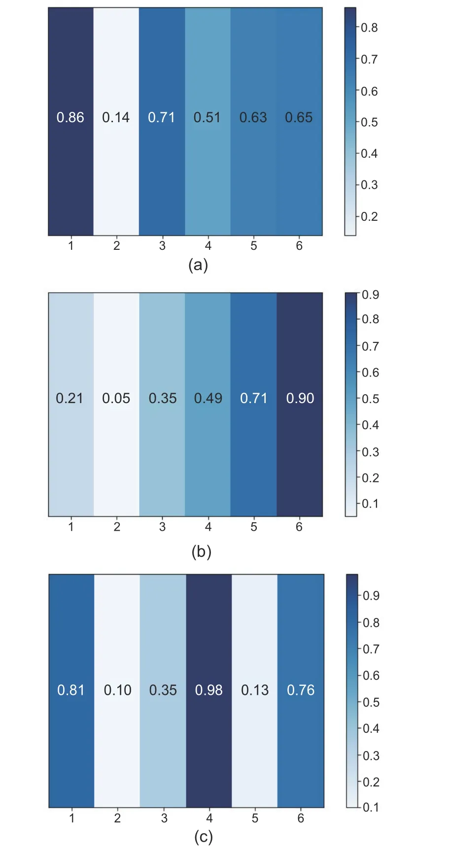
Fig.4 The heat map of attention bias on time steps:(a) OBD1; (b) OBD2; (c) OBD3.The numbers in the middle of each subfigure indicate the bias weights at the corresponding time steps

The results of Precision, Recall, and F1 for OBDs at different thresholds are shown in Fig.5.Compared with the no-pruning condition, in Figs.5a and 5b, all metrics were improved for OBD1 and OBD2 after pruning, and the best results were concentrated under the threshold range of 200–300.For OBD3, in Fig.5c, there was no significant change before and after pruning, mainly because its band prediction sequence length was significantly smaller than those of the two other OBDs (PES of OBD3 is 1/2 that of OBD1 and 1/3 that of OBD2).Further,when the length of the sequence to be predicted was small, we found that the correction effect of the pruning strategy was more limited.However, the increasing length of the sequence to be predicted led to an increasing number of contexts with anomalous emissions.Specifically, when the sequence to be identified reached a certain length, the construction strategy can effectively reduce the false positives of pseudo anomalies and increase the robustness of high-emission detection.In addition, for OBD2, we observed that the pruning strategy can improve the evaluation index of high-emission detection, but not over-pruning; namely, the evaluation score of DTW threshold 400 was smaller than 0.When the con-

Table 4 NOx concentration prediction performance on vehicle OBD datasets of different models

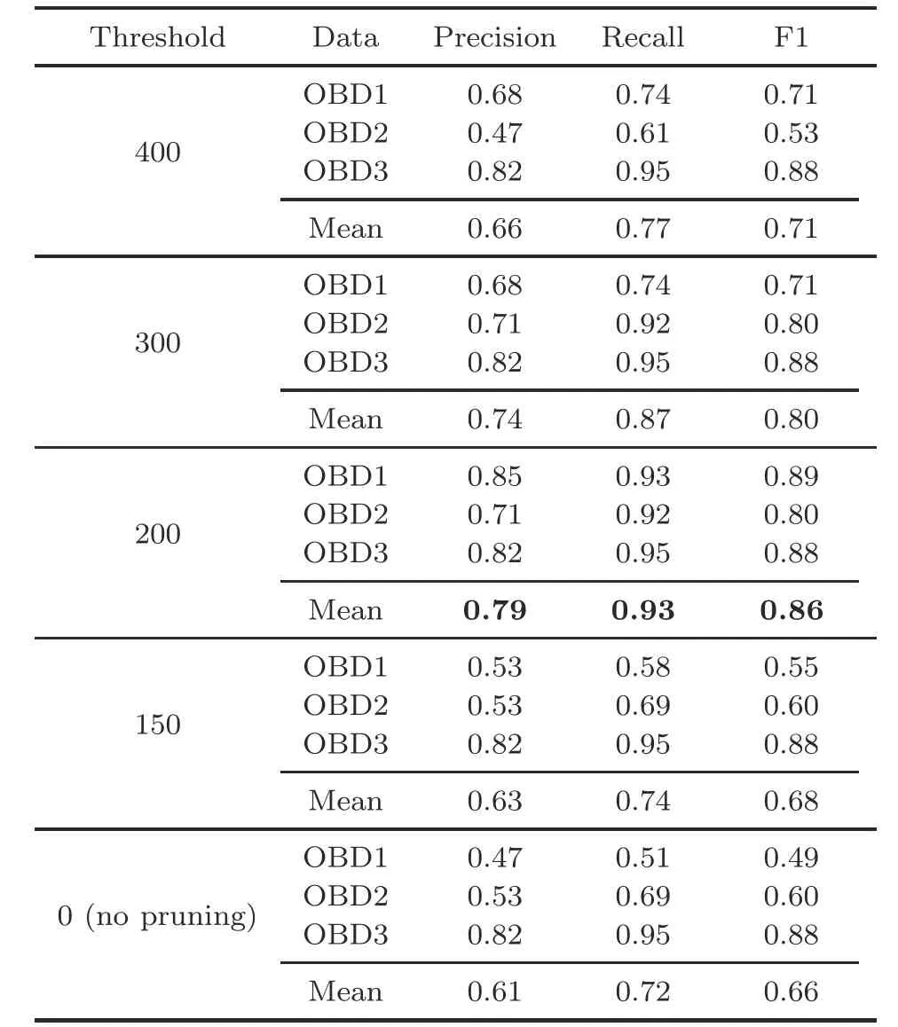
Table 5 Results of contextual anomaly identification with different pruning thresholds for DTW

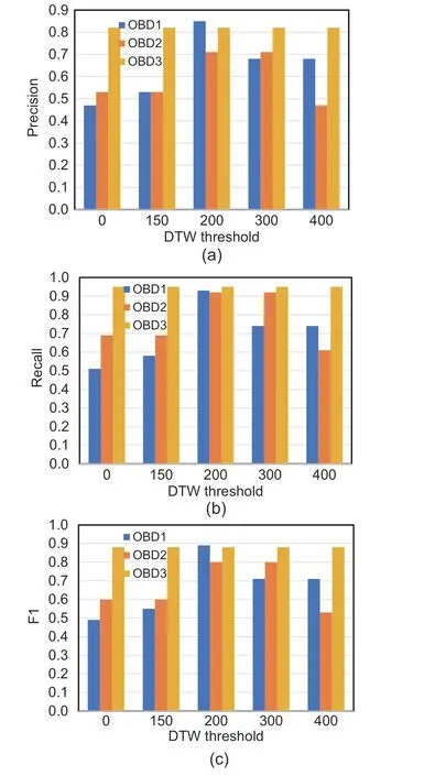
Fig.5 Evaluation visualization of different dynamic time warping (DTW) thresholds for different OBDs:(a) Precision; (b) Recall; (c) F1

structed threshold was too large, the emission error series had low similarity and the true abnormal emission series were incorrectly reclassified to the normal range.This behavior defeats the purpose of pruning.

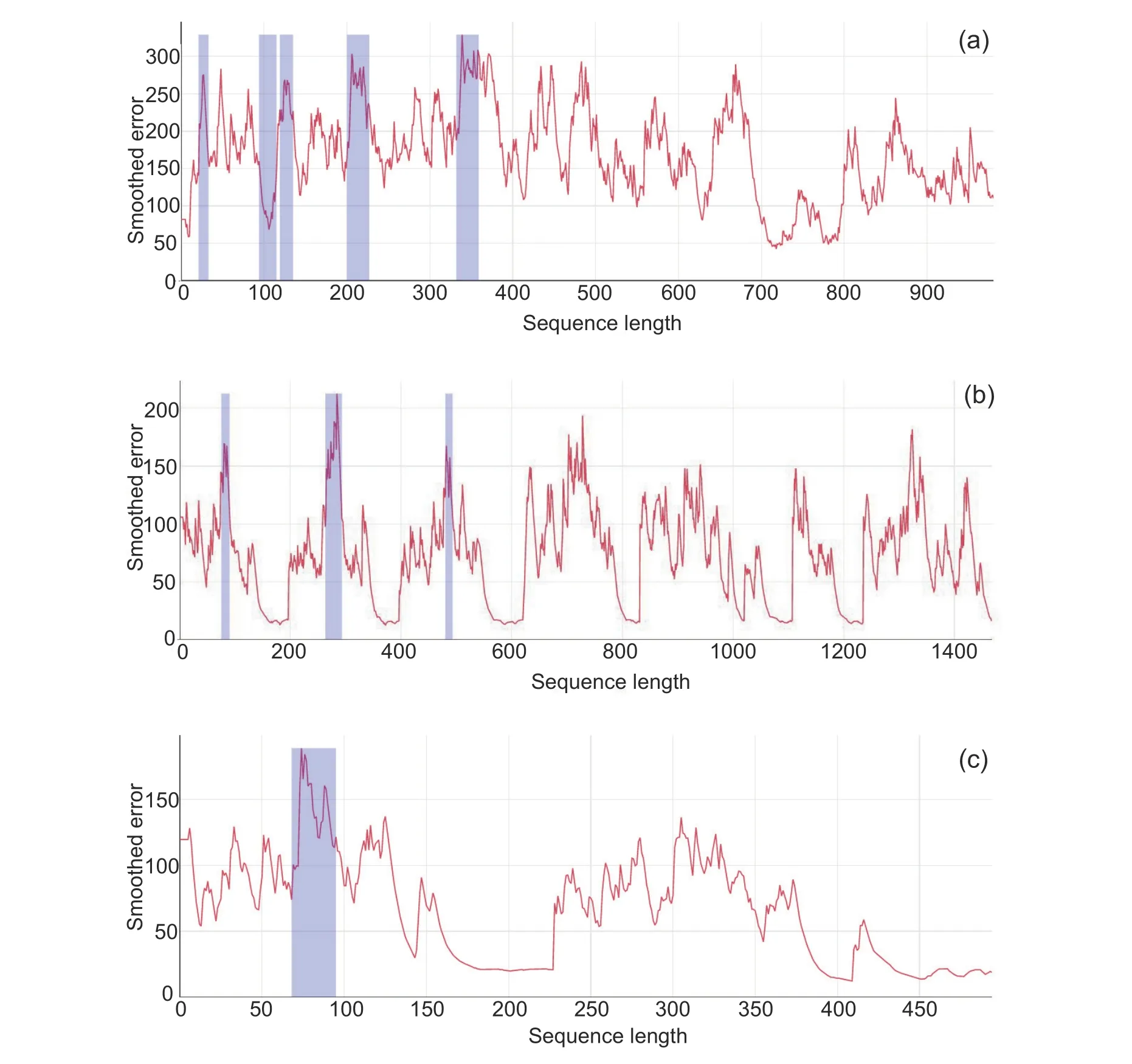
Fig.7 Anomaly identification on the number of emission sequences to be predicted (PES) for different OBDs:(a) OBD1; (b) OBD2; (c) OBD3.The shaded area is the identified abnormal sequence segment

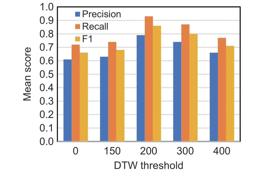
Fig.6 Mean evaluation score of different dynamic time warping (DTW) thresholds for different OBDs

For the trend of the average results of each index, the overall pattern increased and then decreased,and the best recognition effect was obtained for DTW 200 (Fig.6).As shown in Fig.7, for the anomaly emission recognition at DTW 200 of three OBD sequences to be detected, the high-emission identification interval of OBD1 appeared to be concentrated mainly in the time period when the NOxconcentration rised suddenly.A short period of decline followed by a rise was also detected.The highemission identification intervals of OBD2 and OBD3 were concentrated mainly in the spike areas, significantly higher than the front and rear sections.When some error spikes were not very prominent,the model did not determine high emissions.Compared with OBD1,the smoothed error curves of OBD2 and OBD3 were more periodic.This indirectly indicated that vehicle 1 was driving in scenarios with complex conditions(e.g.,rural roads with lack of light),while vehicles 2 and 3 were driving in relatively regular working conditions (e.g., urban roads).Overall, the identification threshold for the high-emission interval was adapted to the context rather than determined over the entire driving period.The TSAO-LSTM prediction errors for different dataset ratios are given in the supplementary materials.

6 Conclusions

In this paper, we propose an unsupervised dynamic threshold discrimination method based on time-series prediction for accurate detection and identification of high-emission vehicles.By establishing driving conditions in continuous time periods, we formulate vehicle emission identification as a time-series anomaly detection problem.First,considering the actual scenario in which various vehicles have attention bias in the prediction time steps, we propose an evolutionary optimized TSAOLSTM emission prediction model, which can better learn the vehicle data characteristics and thus improve the prediction accuracy of emission concentrations.Then, the dynamic anomaly thresholds are calculated to determine the anomalous emission intervals on the prediction error series.Finally, considering the interference of a few mutated values on the prediction, we introduce a pseudoanomaly correction strategy to help improve the accuracy of anomaly identification.Experiments on the Hefei mobile source OBD dataset show that our proposed method is highly accurate in high-emission identification.

In the future, we plan to flexibly adjust the length of a single scan sequence according to the time period of driving conditions,and to explore more accurate ways to detect and identify high emissions.

Contributors

Zhenyi XU designed the research.Zhenyi XU and Renjun WANG processed the data.Zhenyi XU drafted the paper.Renjun WANG helped organize the paper.Yu KANG helped in data control and project management.Yang CAO and Yu KANG provided the funding acquisition and revised and finalized the paper.

Compliance with ethics guidelines

Zhenyi XU,Renjun WANG, Yang CAO,and Yu KANG declare that they have no conflict of interest.

Data availability

The data that support the findings of this study are available from the corresponding authors upon reasonable request.