Sailboat navigation control system based on spiking neural networks

Nelson Santiago Giraldo·Sebastián Isaza·Ricardo Andrés Velásquez

Abstract In this paper,we presented the development of a navigation control system for a sailboat based on spiking neural networks(SNN).Our inspiration for this choice of network lies in their potential to achieve fast and low-energy computing on specialized hardware.To train our system, we use the modulated spike time-dependent plasticity reinforcement learning rule and a simulation environment based on the BindsNET library and USVSim simulator.Our objective was to develop a spiking neural network-based control systems that can learn policies allowing sailboats to navigate between two points by following a straight line or performing tacking and gybing strategies,depending on the sailing scenario conditions.We presented the mathematical definition of the problem, the operation scheme of the simulation environment, the spiking neural network controllers,and the control strategy used.As a result,we obtained 425 SNN-based controllers that completed the proposed navigation task,indicating that the simulation environment and the implemented control strategy work effectively.Finally,we compare the behavior of our best controller with other algorithms and present some possible strategies to improve its performance.

Keywords Sailboat·Control·Spiking neuron·Reinforcement learning·BindsNet·USVSim

1 Introduction

Research on autonomous navigation systems (ANS) for unmanned vehicles has become a popular topic, particularly in relation to ANS for sailboats due to their primary source of propulsion being wind—a free,abundant,and ecofriendly resource.Sailboats have shown great potential for long-term navigation and marine monitoring applications where they cannot touch land for extended periods, making the energy efficiency of their different systems essential.However,designing an ANS for sailboats is challenging due to complex sailboat dynamics and the variability of wind and waves[1,2].Several authors have suggested controllers for ANS that require deep knowledge of sailboat dynamics.Abrougui et al.[1] designed an automatic control system to control heading and sail opening based on sliding mode control.Melin et al.[3] designed a sailing control system for small-scale sailboats, using the field potential control strategy as inspiration.However,acquiring a comprehensive knowledge of dynamic sailboat parameters is complex [2].Therefore,some works proposed control strategies from perspectives that do not require dynamic models.Viel et al.[4]proposed a position-keeping controller using geometric laws.Junior et al.[5]used the Q-Learning reinforcement learning algorithm to solve the path planning problem.Cheng et al.[6]combined a coarse-to-fine strategy and a Q-Learning algorithm for an obstacle avoidance controller.Our work belongs to this category of controllers.

Spiking neural networks(SNNs)have been widely used in neuroscience and more recently,in robotics.Unlike artificial neural networks, SNNs communicate using short electrical pulses distributed over time, known as action potentials or spikes, making their behavior similar to that of biological neurons [7, 8].SNNs are considered a promising solution for various control challenges in robotics since they realistically mimic the underlying mechanisms of the brain,while saving energy and sometimes allowing for simple hardware implementation [7, 9].Recently, research groups and semiconductor sellers have developed specialized neuromorphic hardware,such as Loihi,SpiNNaker,and TrueNorth,to efficiently run SNNs [10].These platforms allow for large SNNs to run with minimal response latency and power consumption, making SNNs an AI technique with a potential in applications where energy and latency are limiting,such as sailboat control tasks[11].Furthermore,the use of SNNs presents an excellent opportunity to move towards a greener artificial intelligence paradigm[10].

Several works in robotics have applied SNN-based controllers to various control tasks.In mobile robotics, Chao et al.[12] used a biological-based recurrent SNN with a leaky integrate and fire(LIF)neuron model[8],spike-timedependent plasticity (STDP) learning rule [13], and rate coding to solve the path planning problem for a drone.Bing et al.[14] used a 32x2 feed-forward SNN with LIF neuron model,ReinforcementSTDP(RSTDP)learningrule[15,16],and rate coding to control a two-wheeled vehicle in a lanekeeping application.Feng et al.[17] used a feed-forward SNN with LIF neuron model,STDP learning rule,and population coding[18]to implement a pain mechanism for the humanoid robot Nao,to solve two tasks:the alerting actual injury task and the preventing potential injury task.In these works,the authors demonstrated that SNNs offer a promising solution for controlling robots with high biological plausibility and good performance.However,due to their complex construction and optimization,SNNs can be challenging to use in a given robotic application.Therefore,SNNs have not yet been extended to many potential applications.It is essential to highlight that there is still no unified framework for the design of SNNs [19].For each application, it is possible to choose different topologies, neural models, learning rules,and coding methods.To the best of our knowledge,no work has addressed the topic of navigation control systems for sailboats using SNNs.In this context,our work is novel in that we applied SNNs to a task in which they had not been previously used, using a reinforcement learning rule.This approach allowed us to train SNNs without knowing the dynamic sailboat parameters and without the need for a sailing database.

In this study,our objective was to devise a control system for sailboats using SNNs and conduct simulations to evaluate its effectiveness.To achieve this,we introduced a design methodology and utilized it to construct various SNN-based ANS.After training and testing these systems,we compared the most effective one with the Viel [2] and USVSim [20]algorithms.We discovered that our control system is operational and improves the deviation error of the USVSim algorithm,but further refinement is necessary to match more advanced algorithms like Viel.The primary contribution of thisstudyisourdesignmethodology,theapplicationofSNNs in sailboat control,and the obtained results,which provide a foundation for future research in this area.

The paper is structured as follows: Sect.2 details the methodology utilized to implement the system.In Sect.3,we provide a description of the sailing problem.Section4 discusses the simulation environment.In Sects.5 and 6,we present the architecture of the SNN and the SNN-based control strategy, respectively.Sections7 and 8 showcase the experimental setup and simulation results.Finally,in Sect.9,we discuss our conclusions and future research.

2 Methodology

In this paper,we introduce an SNN-based ANS for sailboats,along with the simulation environment used for training and testing.Our work comprises the following steps:

1.We developed a simulation environment by integrating the USVSim simulator [20] with our proposed control environment.

2.We defined the SNN architecture, control strategy, and training methodology.

3.We established the training and testing scenarios and explored the design space of various hyper-parameters related to the SNN architecture and control strategy.

4.We trained multiple SNN-based ANS controllers and evaluated their performance in terms of deviation error,total sailing time and total input neurons.

The initial stage of this project involved creating a simulation environment.To achieve this,we made some modifications to certain files in the USVSim simulator [20] and integrated it with a control environment that we developed using the BindsNET library [21].A more comprehensive explanation of the simulation environment is presented in Sect.4.

After ensuring the simulation environment was operational, we proceeded to define the SNN-based controllers required to implement the ANS using the available actuators in the sailboat: the sails and rudder.This involved defining the SNN’s architecture,learning method,and designing the control strategy.We specified various SNN characteristics,including the neuron model,topology,input encoding,and output decoding.In addition,we employed the MSTDP learning rule [16] to train the SNN controllers.Finally, we established reward functions for each SNN, based on the desired maneuvers for the sailboat.A detailed explanation of the SNN’s architecture is provided in Sect.5.

While designing the SNN-based controllers, we discovered several hyperparameters that influenced the behavior of the ANS controller.Therefore,we explored the design space of these parameters to identify a set of controllers that minimized both the deviation error and the total sailing time.A more detailed explanation of the control strategy is provided in Sect.6.

As a last step, we created training and testing scenarios for the SNN-based ANS and used them to carry out the design space exploration.For each design point, we trained and tested each pair of controllers,varying the hyperparameters to obtain different performances.We eliminated designpointswherethecontrollersdidnotcompletethetraining or testing sequence within a specific time frame.Next,we evaluated the performance of the remaining controllers by identifying the set of Pareto optimal controllers.Finally,we chose our best controller and compared them with other sailboat control algorithms.We conducted these experiments on a workstation using Docker v4.3.2[22],with multiple containers running instances of the simulation environment.A more detailed explanation of the experiments is provided in Sect.7.

3 Problem description

An autonomous navigation system(ANS)presents a control challengewhereavehiclemustperformtaskslikefollowinga route,detecting or avoiding obstacles.For the purpose of this work,we limit our focus to the first task:following a route.A route in our study comprises a set of coordinates that the sailboat must reach sequentially.To solve the proposed ANS problem,two critical elements of sailing must be controlled:the rudder,which alters the sailboat’s heading,and the sails,which harness energy from the wind to propel the sailboat.To achieve this,we implemented two SNN-based controllers-one to control the rudder and the other to control the sails.Table 1 shows the input variables(setpoint),sensed variables(feedback),and position orders(control actions)used in our control system.

Besides the variables listed in Table 1,it is crucial to establish the values ofθand|Δr|.These quantities represent the desired heading and the distance between the sailboat and the target point,respectively.We can express these values in terms of the variables given in Table 1,as shown in Eqs.(1)and(2).

Fig.1 Sailboat with its different environment variables

With these variables, we can describe the problem of autonomous navigation mathematically.The aim is to move a sailboat located at(x1,y1) to a position(x,y) using a global true windτand a specific control simulation timet.To accomplish this,the sailboat’s heading must approach the desired heading(ideallyφ=θ)or perform the tacking or gybing maneuvers by executing actionsα1andα2on the rudder and sails,respectively.We assume that the sailboat has reached the target if|Δr|≤kr,wherekris a constant parameter.Figure1 depicts a sailboat with all the aforementioned variables.

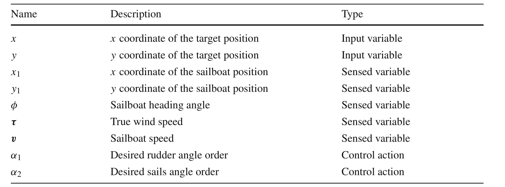
Table 1 External variables to the control system

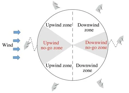
Fig.2 Sailing scenarios and regions

3.1 Sailing maneuvers

Depending on the true wind direction and the target point’s position,the sailboat may face six primary sailing scenarios,as depicted in Fig.2.Our aim was to train the SNN-based controllers to enable the sailboat to move in any direction,and we used these scenarios to define the training and testing scenarios.

To train the SNN-based ANS,we relied on conventional sailing strategies rather than proposing novel strategies.As shown in Fig.2, these sailing strategies can be categorized into two groups: if the sailboat’s heading towards the target point is in the upwind or downwind zones, the sailboat will pursue a straight trajectory to the target.If the sailboat’s heading towards the target point is in the no-go zones,it will perform tacking and gybing maneuvers to reach the target,because a straight trajectory is unfeasible[23].

3.2 True and apparent wind

Understanding the concepts of true wind and apparent wind is fundamental in sailing.The relationship between true windτ,which is the wind perceived by a stationary observer,the apparent winda,which is the wind perceived by an observer inside the sailboat[24],and the sailboat speedvis presented in Eq.(3).

Using Eq.(3)and applying trigonometric and vector laws,we can derive Eqs.(4)and(5)to calculate the apparent wind speedaand directionγaover the sailboat.

3.3 Reinforcement learning

Reinforcement learning is an artificial intelligence technique that differs from supervised and unsupervised learning as it aims to learn what actions to take based on a numerical reward signal.To develop and understand our control strategy,wedefinedsomereinforcementlearningconcepts,which are drawn from[25]:

• Agent The agent represents the actuator controller in terms of control theory.It is the learner and decisionmaker.We define two different agents in this paper:the rudder controller and the sails controller.

• Environment Everything external to the agent can interact with it.

• Action The action represents the control signal in terms of control theory.It is the chosen decision by the agent for a given environment state.In this paper,α1represents the rudder control action,andα2represents the main and jib sails control action(with both sails use the same control action).

• Environment state The environment state represents an environment feedback signal in terms of control theory.It is an indicator that provides information about the environment at a given time.In this paper,Θ1represents the rudder environment state,andΘ2represents the sails environment state.

• Policies A policy generates actions based on the perceived environment states.It defines the way the agent behaves at a given time.In this paper,the policies are the set of all synaptic weights of the SNN-based controllers.

• Reward The reward is a numeric value that aims to rate how good or bad the agent’s actions are within the context of the problem to be solved.We have denotedR1andR2as rewards for the rudder and sail controllers,respectively.

4 Simulation environment

The simulation environment serves as the software infrastructure for training and testing the SNN controllers within the context of an ANS for a sailboat,enabling us to train and run SNNs while also modeling the sailboat and environmental forces acting on it.

For this purpose,we opted for USVSim,an open-source simulator for unmanned surface vehicles (USVs) developed by Paravisi et al.[20].USVSim employs Python 2.7,ROS Kinetic, and Gazebo 7.0.Among the sailboat simulators available,USVSim was selected for its highly detailed physical simulation,including the modeling of environmental disturbances such as winds, water currents, and waves.We customized the default sailboat model provided by USVSim to resemble the physical sailboat we have for future real-world implementation.A list of the modifications is presented below.

• We added a second sail for the sailboat.

• We changed the sailboat’s hull dimensions and mass.

• We changed the sailboat’s rudder dimensions and mass.

• We changed the sailboat’s sails dimensions and mass.

• We changed the sailboat’s environment.

• We changed the USVSim launch characteristics.

On the other hand,we used Python 3 and the BindsNET library[21]to implement our controller environment.BindsNET is a Python 3 library used to simulate SNNs on CPUs or GPUs using PyTorch Tensor functionality.We chose BindsNET for its high-level abstraction, which enables us to describe the behavior of SNNs directly.Below is a list of the tasks performed within our controller environment.

• Make SNN-based controllers with BindsNET library.

• Execute the control system presented in Sects.5 and 6.

• Generate the target points of the training and testing scenarios.

• Execute and save relevant information from the different experiments.

We had to isolate USVSim and our controller environment due to the incompatibility between the Python versions they use.To establish communication between them, we developed a communication link via Socat[26].Finally,we loaded the input data through a configuration file, which contains necessary information to configure our SNN-based ANS,such as control hyper-parameters and SNN topology.

The simulation environment operates as follows: Input data is loaded, the controller environment is configured,and Socat communication is established.At each simulation time step, data arrives from USVSim, and a controller environmentstepisexecuted,whichcanbeatrainingorinference step.This step involves encoding the sensed variables(Sects.5.2 and 6), calculating training rewards (Sects.6.1.3 and 6.2.3),training(or inferring)the SNNs with the encoded variables, decoding the control actions at the SNNs output neuron(Sects.5.4 and 6),and sending them back to USVSim.Figure3 presents the block diagram of our simulation environment.

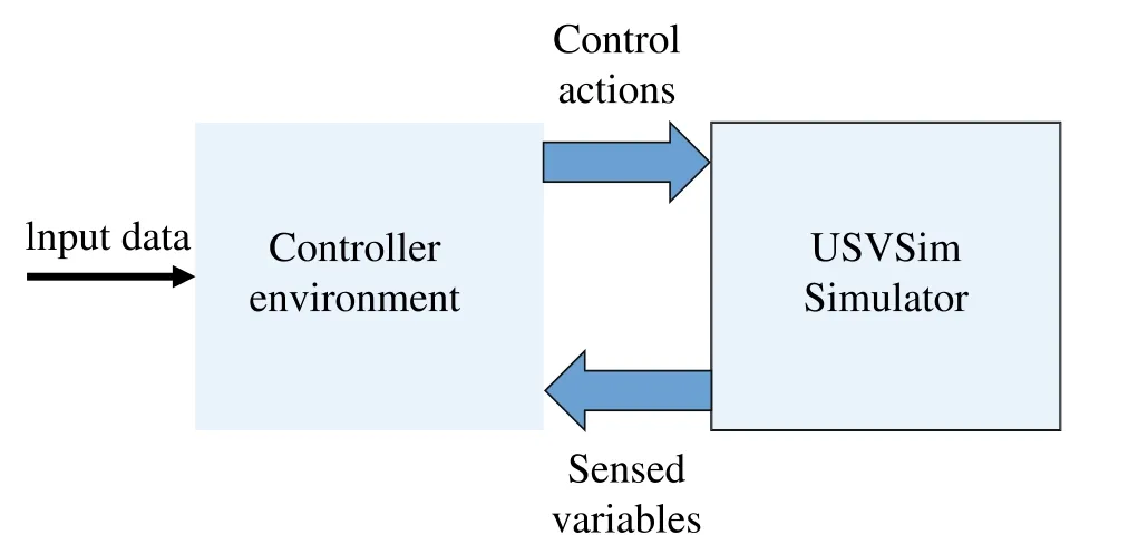
Fig.3 Blocks diagram of the developed simulation environment

5 SNN-based controllers

We developed two SNN-based controllers,one for the rudder and another for the sails,as described in Sect.3.Both SNNs were built using the same approach,which is detailed in this section.

5.1 Neuron model

The neuroscience community has proposed various neuron models for SNNs with different trade-offs between biological plausibility and computational complexity.We chose the leaky integrate and fire(LIF)model[8]due to its simplicity and previous use in other robotics applications[14,27,28].Both SNNs in our study used the LIF model with the default parameters set by BindsNET.

In the LIF neuron model, the axon membrane is represented by an electrical circuit comprising a capacitorCin parallel with a resistorR,which models the cell membrane’s capacitance and leakage resistance.An input currentIext,which is the sum ofIC(current through the cell membrane)andIR(ion diffusion leakage current)components,is applied to the circuit[8].This behavior is described by Equation(6).

In this model, the action potential form is not explicitly described.Instead, spikes are formal events characterized by a“firing time”t f.The firing timet fis determined by a threshold criterion as shown in Eq.(7),and immediately aftert f,the potential resets to a valueVrestless than the threshold potentialϑ[8],as shown in Eq.(8).

5.2 Encoding technique

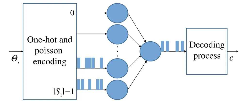
Fig.4 Final block diagram of our SNN architecture

We used an encoding technique to transform the input data into spike trains that can be processed by the SNN.Specifically,we transformed the values of the environment variablesΘ1andΘ2into spike trains using the state encoding approach proposed by Fremaux et al.[29]and Mahadevuni et al.[27].This coding scheme is a form of one-hot coding[30],where only one“hot”set of spiking neurons is excited at any given time.We describe the encoding scheme mathematically in general terms,considering that variables with subscripti=1 belong to the rudder,and withi=2 belong to the sails.

Let us assume that our state variableΘi(Sect.3.3)has a finite number of possible values and can only be in one value at a given time.We define the ascending ordered setSiand its indexni∈Z+(starting from zero),which contain all the possible values of the variableΘi.To each state value, we associated a set of two input spiking neurons and use thenivalue to decide which pair of neurons are excited with a spike train.For instance,if the rudder SNN has four input neurons,n1can take the values 0 and 1.Ifn1= 0, neurons 0 and 1 are excited, and ifn1= 1, neurons 2 and 3 are excited.Thus,at any time,only two input neurons are activated.To excite a neuron,we generated a train of Poisson spikes at a rate of 240Hz in a time window of 500ms.A Poisson spike train is a set of spikes distributed in time,whose firing time is calculated by the Poisson probability distribution[10].In this paper,Θiprovides information about the sailboat’s current state and depends on the sensed variables.We explained how to use these concepts in our study problem in Sects.6.1.1 and 6.2.1.

5.3 SNN topology

Figure4 depicts the architecture of the SNNs,which consist of two fully connected feed-forward layers.The input layer of each SNN is composed of 2|S1| and 2|S2| neurons, corresponding to the rudder and sails,respectively.The output layer comprises a single neuron that generates the control action to be executed by the agent.

Oh, cried the Prince, not one of you is good for anything at all! There is a beggar-girl sitting outside the window, and I ll be bound that she can wash better than any of you! Come in, you girl there! he cried

5.4 Decoding technique

To use the SNN’s output as a control action, we need to decode the spike train into a scalar.We adopted a rate-coding approach[9]for this purpose.Kaiser et al.[28]proposed a decoding method based on the output spike rateOof a neuron and the maximum spike rate of the same neuronOM.They used the ratio ofOtoOMto obtain a number between 0 and 1,as shown in Eq.(9).

as explained in Sect.5.2, for any given environment state,only one set of two neurons is fired at a time for each SNN.With this in mind,the value ofOMis calculated as follows:

• Create an SNN with the topology described in Sect.5.3 and the maximum default weights defined by BindsNET.

• Feed a set of two input neurons with spikes.

• Count the number of output spikes,which isOM.

• Randomize the SNN’s weights and start training.

TheOMcalculationwasperformedonlyoncebeforetraining since it is a constant value in both training and inference stages.We explained how to convert the numbercinto the control actionsα1andα2in Sects.6.1.2 and 6.2.2.

5.5 SNN learning

The selected learning rule for training SNN-based controllers was Dopamine modulated spike time-dependent plasticity(MSTDP),as presented by Florian[16]and Izhikevich[15].This reinforcement learning rule has been used in various robot control applications,such as those developed by Evans[31]and Clawson et al.[32].

MSTDP enables the learning of SNNs by modifying the synaptic weightWabbetween a presynaptic neuron(source)aand a postsynaptic neuronb(target).Mathematically,the change in the synaptic weightWabis the result of modulating the STDP learning rule[13]by a constantR,known as reward[16].The behavior of this learning rule can be observed in Eq.(10),where the variation of the synaptic weightWabis presented in terms of the change of the synaptic weightsPabcalculated by STDP.Our work used the MSTDP learning rule provided by the BindsNET library without any modifications to the default values assigned by the library for the STDP hyperparameters.

6 Control strategy

To develop the rudder and sails controllers,we defined various sailing scenarios that the sailboat must navigate,as well as designs for the rudder and sails controllers, along with training and testing scenarios for the experiments.

6.1 Rudder controller

In this paper, the rudder controller is based on an SNN with the architecture explained in Sect.5.In this section,we definedΘ1,α1and the reward mechanism used.

6.1.1 Input state

We defined the state variableΘ1based on the input variable of the low-level controller proposed by Viel et al.[2].Their controller positions the rudder to compensate for heading disturbances caused by waves and wind,using the difference between the current headingφand the desired headingθas an input variable.Therefore,we setΘ1=θ-φ,whereθis calculated as shown in Eq.(2).

As explained in Sect.5.2,the neurons to be fired depend on the value ofn1.Thus,we derived an equation to calculate it.Assuming that -Θ1MandΘ1Mrepresent the minimum and maximum possible values ofΘ1, respectively.We setn1= 0 whenΘ1= -Θ1Mandn1= |S1|-1 whenΘ1=Θ1M, where |S1| is the cardinality of the setS1(Sect.5.2).In Equation (11), we present a rounded linear model that satisfies these conditions.We rounded the equation to ensure thatn1∈Z+.

In this paper,|S1|represents the number of possible values ofΘ1.For instance, if |S1| = 3 andΘ1M= 90, thenΘ1can take on the values{-90,0,90},andn1can take on the values{0,1,2},respectively.It is important to note that the value of |S1| can impact the controller’s performance, and we,therefore,considered it a controller hyper-parameter.

6.1.2 Output

In Sect.5.4,we explained that the output variablecrepresents the normalized control action calculated by the SNN.To convertcto the rudder control actionα1,we use the following method.

Let -α1Mandα1Mdenote the minimum and maximum possible values ofα1,respectively.If we divide the interval[-α1M,α1M] intoJ1sub-intervals, the size of each subintervalβis given by Eq.(12).

To ensure that the possible values ofα1correspond to the mean value of each sub-interval,it was necessary to restrictcto only takeJ1possible values.To achieve this,a new variablec1was introduced,which is defined in Eq.(13).

To determine the value ofα1for a given intervalc1, we can use the following expressions:Nu=-α1M+β·c1andNu+1=-α1M+β·(c1+1),which correspond to the maximum and minimum points of the intervalc1, respectively.Then,the expression forα1is given by Eq.(14).

By substituting Eqs.(12)into(14),we obtained a simplified expression for computingα1, as presented in Eq.(15).We specify thatJ1should be an odd number,as it allows forα1=0 to be a possible value.

In this paper,J1represents the number of possible rudder control actions andc1represents the index predicted by the SNN.For instance,ifJ1=3 andα1M=90,thenα1can take on the values{-60,0,60}.If the SNN predictsc1=2,thenα1=60.It is important to note that the value ofJ1can impact the controller’s performance.Therefore,we considered it as a controller hyper-parameter.

6.1.3 Reward strategy

As explained in Sect.5.5, our SNN-based controllers were trained using the MSTDP algorithm, which required us to derive an equation for the reward valueR1.To do so, we referred to the results obtained by Florian[16].In their study,an SNN with a rate-decoded output neuron was trained to solve the XOR problem,and they defined the reward asR={-1,0,1}, whereR= 1 indicated an increase in the firing rate of the output neuron,R=-1 indicated a decrease,andR= 0 indicated no change in the firing rate was desired.Based on this,we definedR1∈[-1,1].

ToderiveanequationforR1,wefirstdefinedtheascending ordered setE1(named error set)and its indexe1∈Z+(starting from zero),which contained the results of subtracting all possible values ofα1.For instance,ifJ1=3 andα1M=90,thenα1can take on the values {-60,0,60}, resulting inE1= {-120,-60,0,60,120}.Note that |E1| = 2J1-1 since the possible values ofα1are separated by a fixed distance(Sect.6.1.1).If the elements inE1represent the possible errors between the current heading and its desired value,thenR1must try to make the error zero.Ifez=J1-1 represents the value ofe1corresponding to the error zero, we expect thatR1= 1 ife1-ez=J1-1 andR1= -1 ife1-ez=-(J1-1)due to symmetry with respect to zero.We presented a linear model satisfying these conditions in Eq.(16).

To derive an equation fore1, we introduced the variableΔG1, which represents the difference between the actual heading and the desired heading, and a constantI1, which denotes the maximum allowable error forΔG1.Therefore,ifΔG1≥I1,thene1must be at its maximum(2J1-2).Similarly,ifΔG1≤-I1,thene1must be at its minimum(0).For all other cases, we used a rounded linear model (to ensuree1∈Z+).With the above considerations, we presented an equation to computee1that fulfills the aforementioned conditions,as displayed in Eq.(17).

In this paper,we calculatedΔG1=φ-θ,allowing the controller to learn a policy to follow the desired heading.For instance,if we setJ1=3,I1=60 andΔG1takes values of{-50,0,60},thene1andR1can take on the values{0,2,4}and {-1,0,1}, respectively.It is important to note that the value ofI1can impact the controller’s performance,and we therefore considered it as a controller hyper-parameter.

6.2 Sails controller

In this paper,the sails controller is based on an SNN with the architecture explained in Sect.5.In this section,we definedΘ2,α2and the reward mechanism used.

In contrast to the rudder controller,we derived an approximate model of the behavior of a sail to defineΘ2and to reward the SNN.This model determines the angle ¯α2that maximizes the sailboat’s acceleration in the heading directionφ.We assumed that the sailboat depicted in Fig.1 has a rigid sail1Rigid sails maintain their shape regardless of the wind.and moves at a fixed headingφand speedv.

The first step in deriving the model was to find an equation for the magnitude of the apparent wind forceFφin the heading direction.We based our approach on the work of Melin et al.[3].Equation(18)shows the forceFsacting on the sail,whereρis the sail lift coefficient,σis the sail opening angle with respect to the x-axis, ˆΦis a unit normal vector to the sail,γ ais the apparent wind direction,andais the apparent wind speed(see Sect.3.2).

Note that ˆΦis always normal to the sail for any angleσ.For this to hold true, ˆΦmust have cylindrical(azimuthal)symmetry.By using the transformation equations from cylindrical to Cartesian vectors [33], we derived Eq.(19).This represents the force of the apparent wind on the sail in the global coordinate system of Fig.1.

By applying the transformation equations from Cartesian to cylindrical vectors [33] to Eq.(19) and considering the headingφas the opening angle of the coordinate system,we obtain Eq.(20).In this equation, ˆρand ˆψare unit vectors parallel and perpendicular,respectively,toφ.Therefore,Eq.(21)shows the force magnitude in the heading direction.

The second step in deriving the model was to calculate the derivative of Eq.(21)with respect toσand set it equal to zero.By applying the laws of trigonometry and solving forσ,we obtain Eq.(22).This model maximizes the sailboat’s acceleration in the heading direction,meaning that Eq.(22)can be used to advance the heading direction.

Finally, to calculate the angle ¯α2, we used the operation shown in Eq.(23).In this equation,α2Mrepresents the maximum possible value ofα2.It is important to ensure that bothσ-φandσ-φ+πare within the interval[-π,π).

6.2.1 Input state

We based the definition of the state variableΘ2for the sails controller on Eq.(22).Asγa+φis the input variable in this equation,we setΘ2=γa+φ.

To derive an expression forn2,we followed the same procedure described in Sect.6.1.1 and obtained Eq.(24).In this equation,Θ2Mrepresents the maximum possible value ofΘ2and |S2| represents the cardinality of the setS2(Sect.5.2).Similar to the rudder controller,|S2|denotes the number of possible values ofΘ2, and was considered as a controller hyper-parameter.

6.2.2 Output

Using the same procedure as in Sect.6.1.2,we derived Eqs.(25)and(26).In these equations,α2Mrepresents the maximum possible value ofα2,andcrepresents the normalized control action calculated by the sails output neuron.Similarly to the rudder controller,J2represents the number of possible control actions,and was considered as a controller hyper-parameter.

6.2.3 Reward strategy

Using the same procedure as in Sect.6.1.3,we derived Eqs.(27)and(28).In these equations,ΔG2represents the error between the sails control action and the ideal sails control action, andI2represents the maximum allowable error forΔG2.Similar to the rudder controller,we consideredI2as a controller hyper-parameter.

In this paper, we calculatedΔG2as(α2- ¯α2)t-1.The subscriptt-1 indicates that the value ofα2-¯α2is calculated in the previous simulation instant.Thus,the controller learns a policy by approximating the model presented in Eq.(22).

6.3 Tacking and gybing

Tacking and gybing maneuvers are performed when the sailboat is sailing upwind(tacking)or downwind(gybing)and its intended heading falls within the corresponding no-go zone.If the tacking and gybing no-go zones are defined by anglesσ1andσ2, respectively, then the sailboat has its intended heading in the no-go zones if conditions (29) and (30) are met,for tacking and gybing,respectively.In these equations,Δw1=θ-γτ,whereθis the desired heading andγτis the true wind angle(see Sect.3).

To determine the sailboat’s scenario,we use Eqs.(29)and(30).If we substituteΔw1forΔw2, whereΔw2=φ-γτ, and note that the full angular size of the upwind and downwind zones isπradians(see Fig.2),then Eqs.(31)and(32)provide a way to identify the sailboat’s sailing scenario.

Based on the previous equations,we have established the activation conditions for tacking and gybing maneuvers.To activate tacking,Eqs.(29)and(31)must be satisfied.To activate gybing,Eqs.(30)and(32)must be satisfied.To perform these maneuvers,it is necessary to calculate the desired headingθin a different way than the approach described in Sect.3.We calculatedθusing the methods presented in[1]and[2],whereδrepresents the desired sailboat heading relative to the true wind.Equations(33)and(34)allow us to calculateθ, whereδ1andδ2represent the variableδfor tacking and gybing,respectively.

To execute the maneuvers, we employed the following strategy: upon detecting the need to tack or gybe, the controller assigns a value ofθthat is closest to the sailboat’s headingφ,and switches to the nextθwhen the speed limit(vtfor tacking orvgfor gybing)is reached.For the remainder of the trajectory, heading adjustments are generated whenever the velocity limit is surpassed andΔw1changes sign.

6.4 Controller training

Figure5 illustrates the target points for the sailboat controller in the training scenario.The sailboat training problem involves reaching all the points indicated in Fig.5 from the origin point(x0,y0).We divided the training into two stages:downwind and upwind.In both cases, we define the target point as reached whenΔr≤2.This parameter value is reasonable considering the positioning error in some GPS devices.

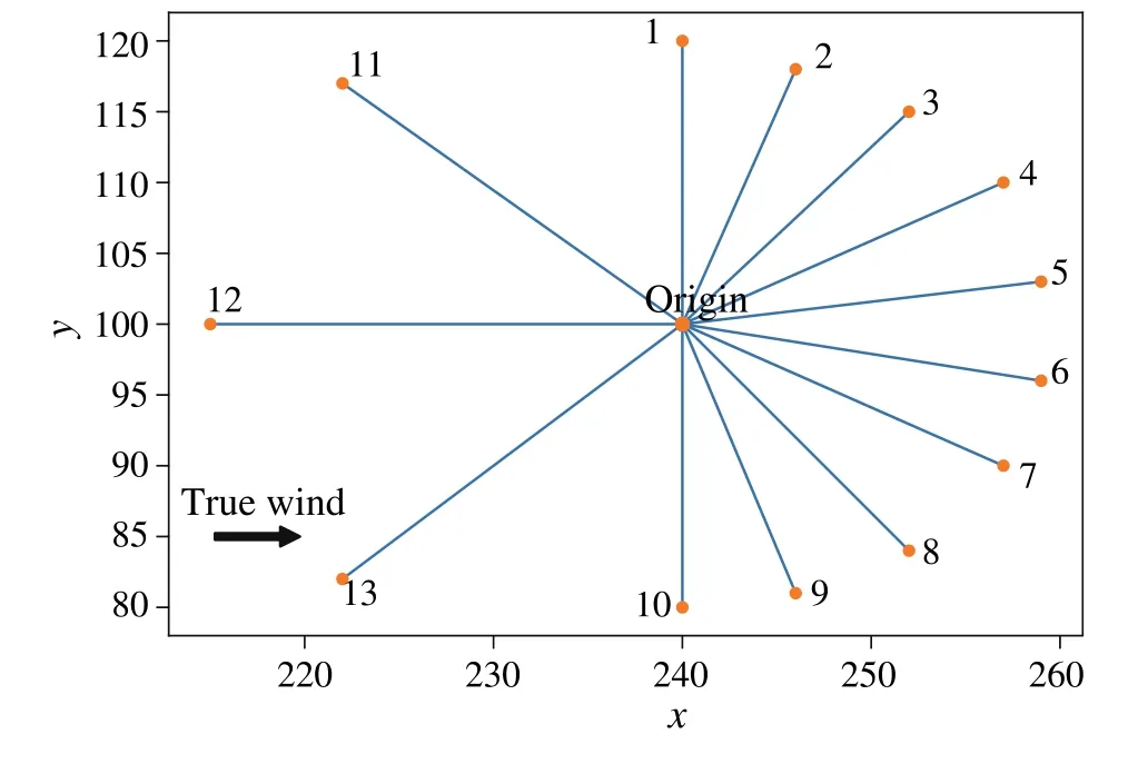
Fig.5 Training scenario for SNN controllers

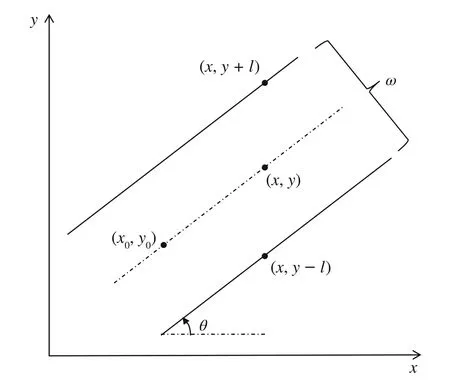
Fig.6 Parallel lane for reset condition

• Downwind In this stage,the SNN-based ANS is trained to learn a suitable policy for moving in the downwind sailing scenario.Points 1–10 in Fig.5 correspond to this stage.

• Upwind In this stage,the SNN-based ANS is trained to learn a suitable policy for moving in the upwind sailing scenario.Points 11–13 in Fig.5 correspond to this stage.

To better understand the following explanation, please refer to Fig.6.To avoid large deviations from the sailboat’s ideal trajectory during the training scenario,we have defined a reset action.This action returns the sailboat to the origin point.When the sailboat deviates from the desired trajectory by a distance of 0.5ω,this action is triggered,and a learning episode ends.In Eq.(35), we presented the logical activation condition for the reset action,wherel= |0.5ωsec(θ)|,θ=arctan(m),andm=(y-y0)(x-x0)-1.If the controller detects a tack or gybe,the point(x,y)is changed to a point in theθdirection(Eqs.(33)and(34)).

To begin the training process, we randomly initialize all weightsWabfor both SNNs.We start on the downwind stage,where the sailboat is positioned at the origin(x0,y0) andφ= 0.If the sailboat deviates a distance of 0.5ωaway from the ideal heading,we trigger the reset action.Similarly,if the sailboat reaches the target point, we trigger the reset action and assign the controller another point(x,y)until the downwind stage is completed.Once the downwind stage is finished,we start the upwind stage,where the sailboat is at the origin(x0,y0) and.Again, if the sailboat reaches the target point, we trigger the reset action and assign the controller another point(x,y)until the upwind stage is completed.In both scenarios,we randomly select the sailboat’s next target point.

In the downwind stage, we setσ2= 0 to ensure that the sail controller responds appropriately whenθ-φ= 0.For the upwind stage, we chose a small value forvtand a large value forδ1to make the tacking turn slow,enabling the sail controller to learn how to respond over a wide range of angles with few points.Specifically,we setvt=0.2,σ1=π,τ=1,andγτ=0.

6.5 Controller testing

In Fig.7, we presented the target points used to test the sailboat controllers.The sailboat testing problem involves reaching all the points shown in Fig.7,following the direction of the arrows.We proposed twelve segments, two for each region of Fig.2.

The testing process is as follows:the sailboat is initially positioned at point 1 with a heading of, and the controller is assigned point 2 as the first target.Once the sailboat reaches a target, the next point in the trajectory is assigned until the sailboat has traveled through all twelve defined trajectories.Similar to the training environment,we consider a target point reached if|Δr|≤2.For this scenario,we selected the following values:σ1=0.5π,, as these values are commonly used for tacking and gybing maneuvers [23, 34].Additionally, we selectedvt=0.47,vg=0.8,τ=1,andγτ=0.

7 Experiments

As a first step for our simulation experiments, we needed to determine the values for the control hyper-parameters.Initially, we were uncertain about what values to assign tothem.Therefore, we performed a manual calibration until we obtained a functional SNN-based ANS.The SNN-based ANS we found has the following parameters:J1=11,J2=15,I1=I2=40◦,|S1|=5,|S2|=18.

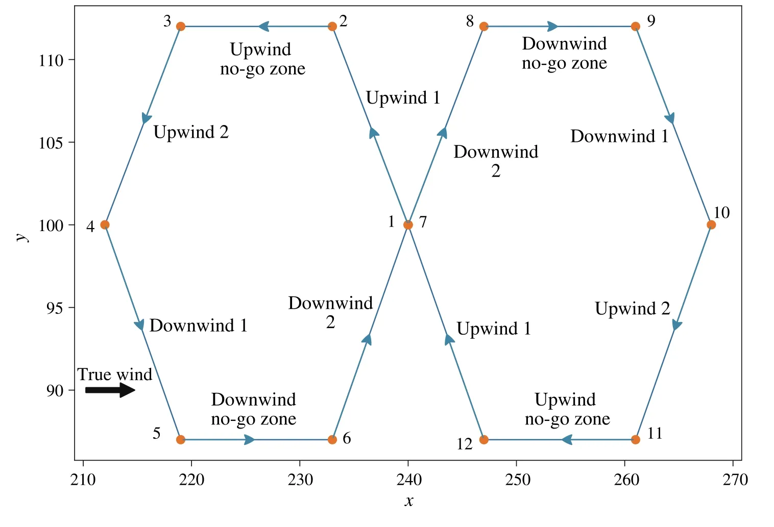
Fig.7 Testing scenario for controllers

For the hyper-parametersJ1andJ2, which can only be odd(Sect.6.1.2),we chose four values:the calibration value,one value above it,and two values below it.We selected four values forI1andI2: the calibration value and three higher values, each separated by 10◦.Finally, we decided that the variables|S1|and|S2|should take two values:the calibration value and its double,in order to double the number of neurons in the input layer and explore more complex SNNs.Next,we present the specific values for each hyper-parameter.

•J1={5,9,11,13}.

•J2={11,13,15,17}.

•I1={70◦,60◦,50◦,40◦}.

•I2={70◦,60◦,50◦,40◦}.

• |S1|={5,10}.

• |S2|={36,18}.

To find out how the behavior of the SNN-based ANS is influenced by different combinations of hyper-parameters,we opted to explore the design space of the SNN-based ANS using the previously selected hyper-parameters.Our aim was to examine all 1024 possible combinations of hyperparameters to identify the SNN-based ANS that executes the testing scenario in the shortest possible time, the smallest deviation error,and the fewest number of neurons.

We assigned an integer value between 1 and 1024 to each possible hyper-parameters combination.These were ordered according to the sequence(J1,J2,I1,I2,|S1|,|S2|).To generate the combinations, we systematically varied all possible values of the hyper-parameters, starting with |S2|and moving towardsJ1.Combinationl= 1 corresponds to(5,11,70◦,70◦,5,36), and combinationl= 1024 corresponds to(13,17,40◦,40◦,10,18).

To evaluate the behavior of various SNN-based ANS in a testing scenario,it is necessary to first train them.Consequently, each experiment entails the training and testing of a single SNN-based ANS.Finally,a Docker image was created to contain the simulation environment for conducting the design space exploration.The exploration was executed on a workstation capable of running up to five experiments simultaneously.Figure8 illustrates the execution scheme for the design space exploration.

8 Results and discussion

Our design space exploration took approximately 13 days to perform the 1024 experiments required to explore the different SNN-based ANS.Out of the 1024 experiments conducted, 88 experiments failed the testing scenario, 511 experimentsfailedthetrainingscenario,and425experiments completed both scenarios correctly.An experiment fails to complete a scenario when it does not reach all target points within 105min for training and 45min for testing.It should be noted that controllers that failed to complete a scenario do not necessarily fail to work;they simply fail to complete the proposed task within the defined time interval and thus will not be considered among the best.

To process the data generated by the design space exploration,we defined three optimization goals:

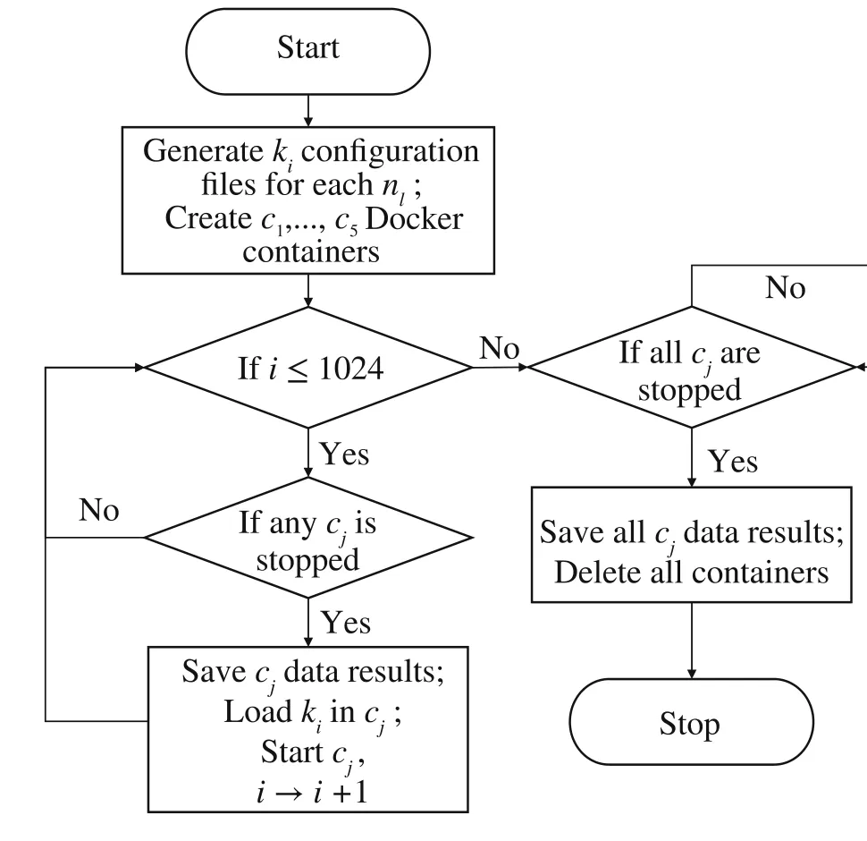
Fig.8 Design space exploration execution scheme

• Sailing time(ts):total time to reach the target in the testing scenario.

• Deviation error (De): mean absolute error between the path traveled by the sailboat and the ideal path in all trajectories except no-go zones.

• SNN size(S):total number of input neuronsS=2(|S1|+|S2|)(as discussed in Sect.5).

The results of thetsmetric are depicted in Fig.9 as a histogram.Each bar in the histogram represents a specific time range.The numbers on the time axis indicate the starting point of the range,and the numbers above the bars represent the total number of experiments.The figure reveals that most test scenarios were completed in under 600s.Moreover,there were 14 experiments that finished in less than 400s,making them potential candidates for the SNN-based ANS with the best time.

Figure10 displays the mean absolute errors(MAE)for the trajectories depicted in Fig.7 (excluding the no-go zones),aiming to observe the behavior of the SNN-based ANS in different trajectories.Most of the trajectories exhibit MAE between 0.3m and 2.1m, while the downwind 1 trajectory has the highest errors,with a considerable number of results positioned to the right of the value 2.1.This indicates the need for further training for downwind 1 trajectories.Notably,some SNN-based ANS exhibit errors per trajectory below 0.4,indicating minimal deviation from the ideal path.

To identify the best controllers of the design space exploration, we calculated the Pareto points [35] by minimizing the metricsts,S, andDeas explained earlier.Figure11 presents the Pareto frontier points,where N_time represents the normalizedtsvariable, N_error denotes the normalizedDevariable,and N_states reflects the normalizedSvariable.Table 2 presents the values of the three target metrics for each Pareto frontier point.

After analyzing the results in Table 2,we have determined that experimentl= 923 is the best performing SNN-based ANS.This is because it belongs to the set of experiments withts< 400, has the lowestDeamong this set, and also has one of the lowestSvalues.

8.1 Comparison with other control algorithms

In this section,we presented comparisons between our SNNbased ANS and other control algorithms found in the state of the art,to solve the same sailing task.

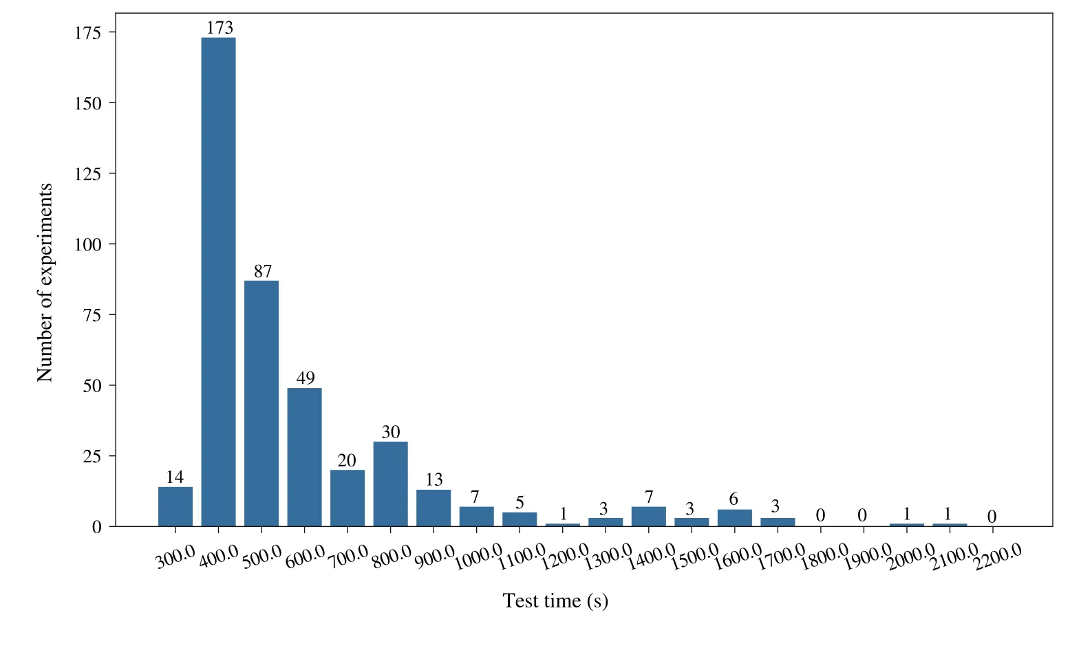
Fig.9 Testing time for the completed simulation points

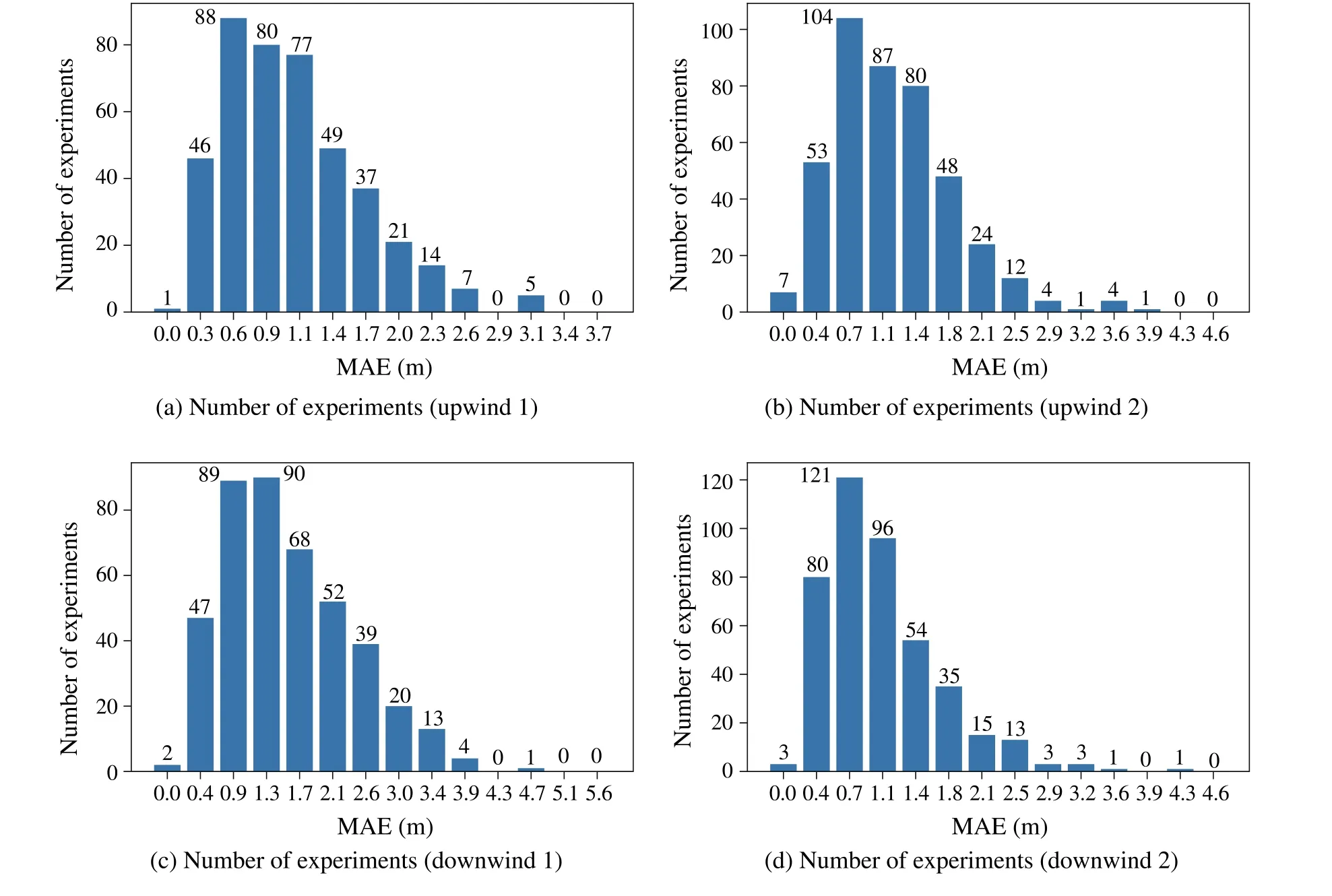
Fig.10 MAE distribution for the different testing trajectories

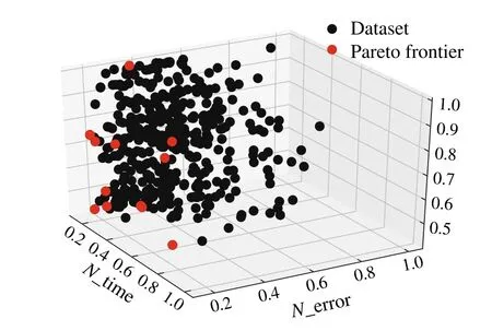
Fig.11 Graphical Pareto frontier representation

In Fig.12, we present the path followed by ourl= 923 SNN-based ANS in the testing scenario (blue line).The different maneuvers performed can be seen in trajectories 2 →3, 11 →12, 5 →6, and 8 →9, where the sailboat tacked and gybed properly as it had to sail in the no-go zones.For the rest of the trajectories,the sailboat reached the target point following the headingθwith small deviations from the green line (lowDe).Based on these observations, we can conclude that ourl= 923 SNN-based ANS learned a suit-able sailboat control policy, and the developed simulation environment is useful for training SNNs.

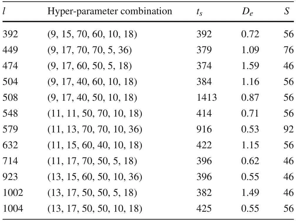
Table 2 Pareto frontier results

For comparison,we selected Viel’s low-level control algorithm [2] and the default sailing algorithm of the USVSim[20].Viel’s algorithm operates based on a geometric approximation of the sailboat’s behavior,and performs corrections to perturbations in the sailboat’s heading.The USVSim control algorithm is a proportional integral controller(PI)calibrated for the original USVSim sailboat.We implemented both algorithms in our simulation environment and ran the testing scenario for each one.

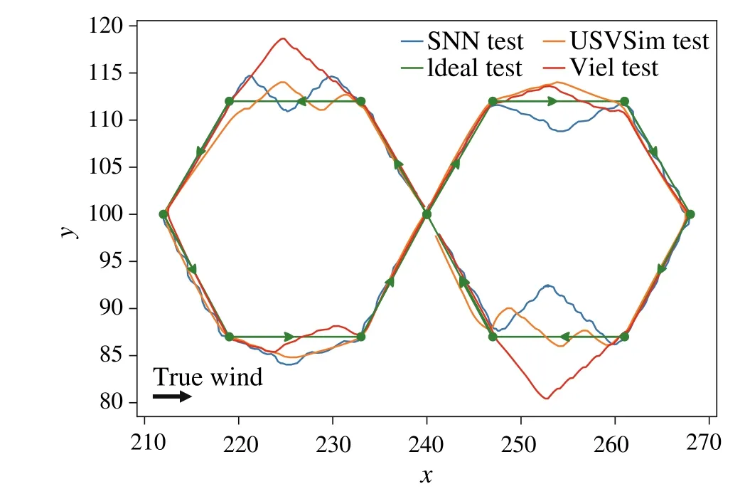
Fig.12 Comparison of the paths followed by the different control algorithms

Table 3 Algorithm comparison metrics

In Fig.12 and Table 3,we present the results obtained by each control system in the testing scenario.All algorithms successfully completed the scenario.Viel’s controller outperformed the other algorithms as it had the smallest travel time and deviation error with respect to the ideal path.While the USVSim algorithm had a better travel time than the SNNbased ANS,the SNN-based ANS had a lower deviation error.These results suggest that although the SNN-based ANS does not perform better than a robust controller like Viel’s,it may be useful as a viable alternative to a PI controller in tasks where low deviation error is important.

It is important to note that this is our first attempt at developing SNN-based ANS.We employed a simple architecture,a specific training,a learning approach,and a particular testing technique.While our results do not exhibit significant improvements over state-of-the-art controllers, there may be other SNN architectures and training methods that can enhance performance in sailing tasks.Thus, these findings can provide a foundation for further exploration and development of SNN-based ANS designs.

9 Conclusion

In this work,we developed an SNN-based ANS for sailboat control.We formulated the sailing problem, identified the SNNs features,developed a control strategy,and established training and testing scenarios.We conducted a design space exploration in a simulated experiments to minimize testing time, deviation error, and total input neurons.Our experiments generated 425 controllers that successfully navigated the testing scenario.Our best controller achieved a testing time of 396s and a deviation error of 0.55m,outperforming the USVSim controller in deviation error.However, it performed worse than the Viel’s controller,which completed the testing scenario in 309s with an error of 0.51m,indicating a need to reevaluate aspects of our methodology.One potential change is to use a reinforcement learning algorithm with an eligibility trace instead of the MSTDP algorithm,as it would enable more advanced reward strategies.Other possibilities include exploring recurrent SNNs to incorporate information about past events,as well as conducting a more comprehensive hyper-parameter search to find optimal values for our sailing task.As future work,we will implement thel=923 SNN-based ANS on a real small-scale sailboat to validate its performance under real conditions.

Author Contributions Ricardo Velasquez conceived the idea of this projectandco-superviseditsdevelopment.SebastianIsazaco-supervised the project development and helped write and review the paper.Nelson Giraldo proposed some of the ideas,developed the codes,run the experiments and wrote the paper.All authors read and approved the final manuscript.

Funding Open Access funding provided by Colombia Consortium.The Authors declare that this work was supported by the University of Antioquia with project PRG2017-16182 and by the Colombia Scientific Program within the framework of the call Ecosistema Científico(Contract No.FP44842-218-2018).

Data availability A repository with the results obtained from the simulations is available at https://github.com/nsantiagogiraldo/Sailboat_simulator.

Declarations

Conflict of interest The Authors declare that they have no conflicts of interest.

Open Access This article is licensed under a Creative Commons Attribution 4.0 International License,which permits use,sharing,adaptation, distribution and reproduction in any medium or format, as long as you give appropriate credit to the original author(s) and the source, provide a link to the Creative Commons licence, and indicate if changes were made.The images or other third party material in this article are included in the article’s Creative Commons licence,unless indicated otherwise in a credit line to the material.If material is not included in the article’s Creative Commons licence and your intended use is not permitted by statutory regulation or exceeds the permitteduse,youwillneedtoobtainpermissiondirectlyfromthecopyright holder.To view a copy of this licence, visit http://creativecomm ons.org/licenses/by/4.0/.