A distributed EEMDN-SABiGRU model on Spark for passenger hotspot prediction∗#

Dawen XIA ,Jian GENG ,Ruixi HUANG ,Bingqi SHEN ,Yang HU ,Yantao LI,Huaqing LI

1College of Data Science and Information Engineering, Guizhou Minzu University, Guiyang 550025, China

2Department of Automotive Engineering, Guizhou Traffic Technician and Transportation College, Guiyang 550008, China

3College of Computer Science, Chongqing University, Chongqing 400044, China

4College of Electronic and Information Engineering, Southwest University, Chongqing 400715, China

Abstract: To address the imbalance problem between supply and demand for taxis and passengers,this paper proposes a distributed ensemble empirical mode decomposition with normalization of spatial attention mechanism based bi-directional gated recurrent unit (EEMDN-SABiGRU) model on Spark for accurate passenger hotspot prediction.It focuses on reducing blind cruising costs,improving carrying efficiency,and maximizing incomes.Specifically,the EEMDN method is put forward to process the passenger hotspot data in the grid to solve the problems of non-smooth sequences and the degradation of prediction accuracy caused by excessive numerical differences,while dealing with the eigenmodal EMD.Next,a spatial attention mechanism is constructed to capture the characteristics of passenger hotspots in each grid,taking passenger boarding and alighting hotspots as weights and emphasizing the spatial regularity of passengers in the grid.Furthermore,the bi-directional GRU algorithm is merged to deal with the problem that GRU can obtain only the forward information but ignores the backward information,to improve the accuracy of feature extraction.Finally,the accurate prediction of passenger hotspots is achieved based on the EEMDN-SABiGRU model using real-world taxi GPS trajectory data in the Spark parallel computing framework.The experimental results demonstrate that based on the four datasets in the 00-grid,compared with LSTM,EMDLSTM,EEMD-LSTM,GRU,EMD-GRU,EEMD-GRU,EMDN-GRU,CNN,and BP,the mean absolute percentage error,mean absolute error,root mean square error,and maximum error values of EEMDN-SABiGRU decrease by at least 43.18%,44.91%,55.04%,and 39.33%,respectively.

Key words: Passenger hotspot prediction;Ensemble empirical mode decomposition (EEMD);Spatial attention mechanism;Bi-directional gated recurrent unit (BiGRU);GPS trajectory;Spark

1 Introduction

With the rapid development of data technology,mobile trajectory big data analytics has become a research hotspot in urban computing and smart cities (Batty et al.,2012;Zheng Y et al.,2014;Zheng Y,2017).In urban transportation networks,Global Positioning System (GPS) equipped taxis play an essential role in our daily life,and the data extracted from the massive taxi GPS trajectories can effectively reflect valuable information,such as passenger hotspot distribution (Bi et al.,2021),passenger travel pattern (Gong et al.,2016),taxi cruising pattern (Xu et al.,2017;Xia et al.,2021a;Zhang WY et al.,2022),and traffic flow distribution (Ali et al.,2021;Seng et al.,2021;Xia et al.,2021b).The practical information mined from taxi mobile trajectory data can provide valuable decisions for passengers,taxi drivers,and traffic managers.Simultaneously,in terms of taxis carrying passengers,some passengers have difficulty in finding taxis in certain places,and some taxi drivers have difficulty in searching for passengers.Moreover,this imbalance between supply and demand may cause severe traffic congestion,wasted resources,decreased profits,and reduced passenger satisfaction (Zheng LJ et al.,2018).Therefore,data interpretation,data manipulation,and data value extraction with big data techniques have become critical issues for intelligent transport systems (ITSs) (Engelbrecht et al.,2015;Zhu et al.,2018).Given this,it is necessary to predict potential passenger hotspots to reduce fuel consumption and cruising time (Dong et al.,2017).

Passenger hotspot prediction has been a hot research direction in smart cities,and researchers have conducted many studies in recent years,which can be divided into two types.Traditional time-series methods are used to predict passenger hotspots (Li XL et al.,2012;Jamil and Akbar,2017;Qu et al.,2019),but they fail to consider non-stationary series and the problem of reduced prediction accuracy caused by excessive differences in values,as taxi GPS trajectory data are non-stationary spatiotemporal data with variability between values.Therefore,it is vital to consider non-stationary data,and their variability is essential.With the rapid development of neural networks,many researchers have used neural networks such as long short-term memory (LSTM) and gated recurrent unit (GRU) to predict passenger hotspots.However,these models are not applied in passenger hotspot prediction (Kim et al.,2020;Li XF et al.,2020;Luo et al.,2021;Yang et al.,2021),and do not consider the backward and forward contextual information either.Furthermore,researchers have used attention mechanisms in neural network models to enhance prediction accuracy.For example,the self-attention mechanism and soft attention mechanism focus only on the correlation of the data without considering the spatial correlation between the map road network and passenger hotspots.In addition,several researchers have employed ensemble empirical mode decomposition (EEMD) combined with traditional models for short-term metro passenger flow and ship movement prediction (Nie et al.,2020;Liu XP et al.,2022),as well as combining neural networks for traffic flow (Gao et al.,2020),metro passenger flow (Cao et al.,2022),and waiting time (Xia et al.,2022a) prediction.However,they combined two methods but did not implement these methods in the Spark distributed framework.

To address the above problems,we propose a distributed ensemble empirical mode decomposition with normalization of spatial attention mechanism based bi-directional gated recurrent unit (EEMDNSABiGRU) model on Spark for passenger hotspot prediction.Specifically,the non-smooth data are smoothed using the EEMDN method.Then,the spatial attention mechanism is used to capture the correlation of passenger hotspots between grids.Therefore,the BiGRU algorithm is fused to predict passenger hotspots,and the prediction results are inversely normalized and superimposed.Finally,we evaluate EEMDN-SABiGRU based on GPS trajectory data of taxis in Beijing,China.The results indicate that the prediction accuracy of EEMDN-SABiGRU is superior to those of the comparable models.

The main contributions of this work are summarized as follows:

1.An EEMDN method is proposed to reduce the influence of non-stationary time series on the prediction performance and to solve the intrinsic mode function (IMF) confusion problem of the EMD algorithm.

2.A spatial attention mechanism is constructed to capture spatial correlation,extract the number of passengers getting on and offin the grid,form the grid’s spatial weights,and improve the performance of passenger hotspot prediction.

3.A BiGRU model is incorporated to deal with the problem that GRU can obtain only forward contextual information but ignores backward contextual information,which improves the accuracy of feature extraction.

4.With the proposed EEMDN-SABiGRU model and the big taxi GPS trajectory data in Beijing,China,passenger hotspots are successfully predicted in the Spark framework.The experimental results demonstrate that the prediction accuracy of EEMDN-SABiGRU is significantly higher than those of LSTM,EMD-LSTM,EEMD-LSTM,GRU,EMD-GRU,EEMD-GRU,EMDN-GRU,convolutional neural network (CNN),and backpropagation (BP).

2 Related works

In this section,we briefly introduce the works related to passenger hotspots and then analyze the problems.Existing works consist mainly of the traditional time-series methods and neural network methods.

2.1 Time-series methods

The time-series analysis method is widely applied to passenger hotspot prediction.Jamil and Akbar (2017) conducted time-series analysis using an automated ARIMA model to forecast hotspot areas for passengers based on historical spatiotemporal data provided by taxi companies.Li XL et al.(2012) proposed a model to delineate urban hotspots and a method based on an improved ARIMA model to predict the number of passengers in urban hotspots in time and space.Qu et al.(2019) investigated a profitable and graphical taxi route recommendation method called adaptive shortest expected cruising route (ASECR),which uses Kalman filter prediction to obtain probability and capacity locality.Xia et al.(2022b) developed a parallel GS-SVM algorithm based on the Spark framework to predict taxi passenger hotspots.The EMD method has also been widely used because of its significant advantage in processing non-stationary data (Huang et al.,2019).Yao et al.(2016) employed the EMD-PSOSVM algorithm to predict safety conditions.Nie et al.(2020) improved the EMD and SVR algorithms for short-term ship motion prediction.In addition,the EEMD method responds to the EMD method’s modal confounding problem.Liu XP et al.(2022) put forward three hybrid forecasting models,EEMD-ARIMA,EEMD-BP,and EEMD-SVM,for predicting short-term urban metro demand changes.Wang et al.(2022) employed an improved EEMD method for active power filter (APF) detection.Qin et al.(2020) proposed an EEMD-LPP model for carbon price prediction.Cheng et al.(2021) presented an EEMD-SVD-LWT denoising algorithm for atmospheric LiDAR.Jiang et al.(2014) used an EEMD-GSVM model for short-term prediction to address the high-speed rail passenger flow prediction problem.

2.2 Neural network methods

In recent years,neural network methods have attracted significant attention in passenger hotspot prediction.Yang et al.(2021) proposed a new wave-LSTM model based on LSTM and wavelets to predict passenger flow.Li XF et al.(2020) investigated a fast correlation filter and an LSTM based on wavelet transform to predict passenger demand in different regions at different time intervals.Kim et al.(2020) designed an interpretable deep learning model to evaluate a quota system that balanced two demanded modes.A two-stage interpretable machine learning modeling framework LSTM was developed through a linear regression (LR) model combined with a long short-term hierarchical neural network.Luo et al.(2021) proposed a multi-task deep learning (MTDL) model to predict short-term taxi demand at multiple regional levels to reduce hybrid bus emission (HBE) while improving efficiency.Li ML et al.(2021) designed a new predictive energy management strategy based on passenger forecasting and exhaust emission optimization.Ou et al.(2020) presented a new deep learning framework,STP-TrellisNets,which augments the emerging temporal convolution framework (TrellisNet) to predict subway station passenger flows accurately by spatiotemporal forecasting.Saadallah et al.(2020) proposed BRIGHT for forecasting demand using a supervised learning framework for perceivable demand.BRIGHT aims to provide accurate forecasts for demand in short term through an innovative timeseries analysis method to deal with different types of conceptual drift.Zhou et al.(2020) put forward the ST-attention model,which uses a multi-output strategy,but does not employ recurrent neural network (RNN) units of learning,to determine ridership demand and periods in key projected city areas during special periods using a spatiotemporal attention mechanism.In addition,the EEMD method was often combined with neural network methods such as the EEMD-LSTM algorithm,which was proposed to predict surface temperature (Zhang XK et al.,2018).Rezaei et al.(2021) constructed the CEEMD-CNN-LSTM and EMD-CNN-LSTM models to predict financial time series.Yu et al.(2021) constructed an EEMD-Conv3d method for soil temperature prediction.Niu et al.(2021) used an EEMD combined with RNN for landslide prediction problems.Liu J et al.(2020) developed an EEMD-DBN model for urban short-term traffic flow prediction.

In the above studies,researchers used timeseries methods to predict passenger hotspots.However,traditional time-series methods do not consider the impact of non-stationary series on prediction accuracy.Furthermore,although the EMD method can reduce the non-stationarity of time series,it still has the problems of end effects and modal confounding.When using neural networks for passenger hotspot prediction,researchers employed the self-attention mechanism to focus on the correlation of the data without considering the spatial correlation between the map road network and passenger hotspots.Although GRU can solve the problems of gradient disappearance and gradient explosion in RNN,the information-dependent GRU method ignores the information context in the road network,with high complexity and a long prediction time.In addition,few researchers used the EEMD method combined with neural network models for passenger hotspot prediction.To this end,in this paper we present a distributed EEMDN-SABiGRU model on Spark to accurately predict passenger hotspots.

3 EEMDN-SABiGRU model

In this section,we describe the EEMDNSABiGRU model in detail.

3.1 Model overview

The prediction framework based on a distributed EEMDN-SABiGRU model includes data preprocessing,model construction,and model implementation as shown in Fig.1.In data preprocessing,the taxi GPS trajectory data are processed by data extracting,data sorting,grid mapping,and data counting.Then,in model construction,the EEMD algorithm with the normalization method is employed to obtain a finite number of IMFs and a residual (Res) sequence,and the BiGRU algorithm with a spatial attention mechanism is used to construct the EEMDN-SABiGRU model.The prediction results are superimposed by inverse normalization.Finally,in model implementation,the EEMDN-SABiGRU model is implemented on the Spark parallel computing framework.

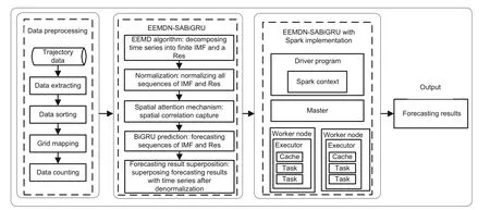
Fig.1 A distributed EEMDN-SABiGRU model on Spark

3.2 Data preprocessing

When collecting taxi GPS data,there are problems such as equipment failure and signal delay,which can cause the collected data to be wrong or missing.For example,some taxi drivers do not update the passenger status in time after picking up a passenger.The data are not collected when the signal is mid-range,and the vehicle passes through a long tunnel.Therefore,it is necessary to remove errors and fill in missing data when processing data to improve the accuracy and reliability of prediction.The process of data preprocessing is illustrated in Fig.2.

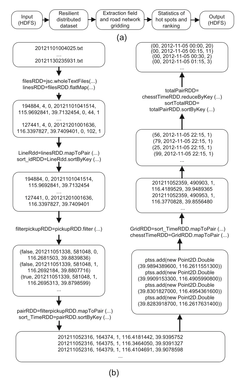
Fig.2 Process of data preprocessing: (a) data preprocessing;(b) data flow

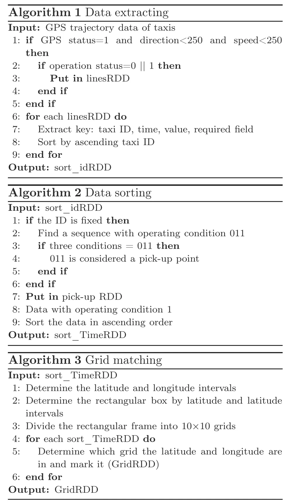
Step 1: data extracting.We first store the data in the Hadoop distributed file system (HDFS) and convert the data into a resilient distributed dataset (RDD) on Spark.We then split the RDD,eliminate the blank and wrong data,and finally extract the required data (taxi identity document (ID),operation status,time,longitude,and latitude).Details are specified in Algorithm 1.

Step 2: data sorting.From the data obtained at step 1,the duplicate IDs are filtered,and the complete 011 passenger-carrying events in the operation status (0 means empty and 1 means passengercarrying) are extracted and sorted in chronological order.Details are illustrated in Algorithm 2.

Step 3: grid mapping.In this work,the latitude and longitude ranges of 39.828 391 87-39.99091533 and 116.261 155 13-116.49543616 are selected,respectively.The sorted data are mapped or matched into these latitude and longitude ranges using the sorted data,and the latitude and longitude of the sorted data gridded as 10×10 are illustrated in Fig.3.Details are described in Algorithm 3.

Fig.3 Road network grid: (a) 10×10 grid;(b) road network with 10×10 grid

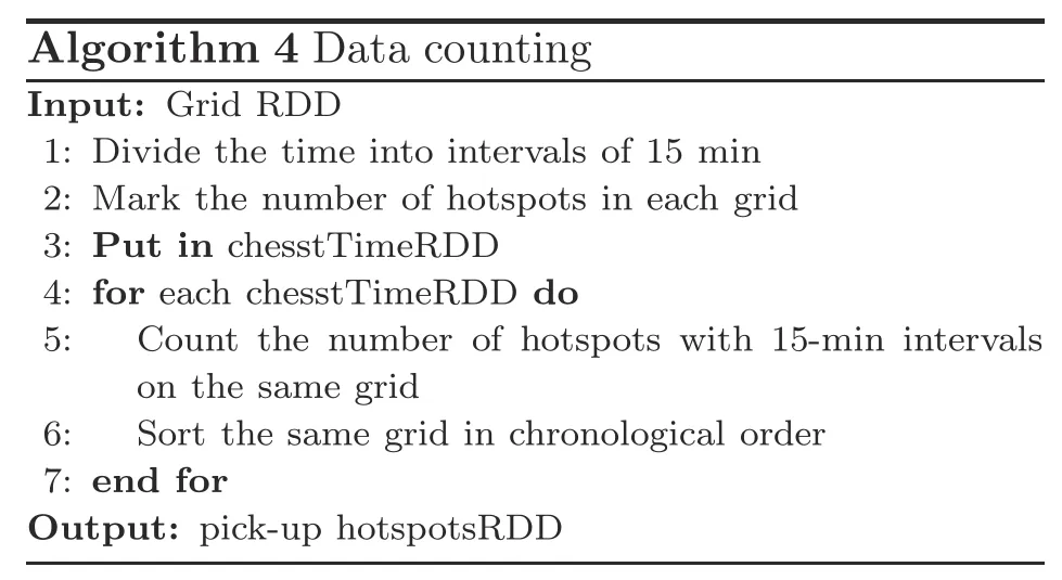
Step 4: data counting.We use the data after mapping the grids,divide them into intervals of 15 min,and count the taxi boarding hotspot data within the same grid at 15-min intervals.Details are given in Algorithm 4.

3.3 Model construction

The process of the EEMDN-SABiGRU model includes three steps: design of the EEMDN algorithm,integration of the BiGRU model,and construction of the spatial attention mechanism.

Step 1: design of the EEMDN algorithm.EEMD,an upgraded algorithm of EMD,smooths the abrupt changes on the time scale by adding white noise to the original signal sequence and adaptively maps the signals at different scales to a suitable reference scale using the uniform distribution of the white noise spectrum.Then,the white noise signal is inputted into EMD for multiple decompositions to obtain the average result,eliminating the noise effect.Finally,the IMF and Res sequences containing a single time scale are obtained,and the IMF and Res are mapped in[0,1]and inputted to the BiGRU model for prediction.The decomposition process is composed of four sub-steps:

(1) Set the total average number of times asM,and add the white noise amplitude signalni(t) with a standard normal distribution to the original signalx(t) to obtain an additional noise signal,which is defined as

wherex(t) is the original signal,ni(t) is theithwhite noise sequence,andxi(t) is theithadditional noise signal.

(2) The noisy signalxi(t) is decomposed by EMD,and the sum of IMFs is obtained,defined as

whereci,j(t) is thejthIMF decomposed after theithwhite noise,ri,j(t) is the residual function,andJis the number of IMF sequences.

(3) Sub-steps 1 and 2 are repeatedMtimes,and white noise signals with different amplitudes are added for each decomposition to obtain the IMF set,which is defined as

(4) The above IMFs are averaged to obtain the final IMF result after EEMD,as shown in Eq.(4),and the IMF and Res obtained by EEMD decomposition are mapped in[0,1].

wherecj(t) is thejthdecomposed IMF.

Step 2: integration of the BiGRU model.The BiGRU model is an improvement of the GRU model,consisting of two unidirectional and opposite GRUs,and the GRU model is defined in Eqs.(5)-(8):

whereztis the updated gate,rtrepresents the reset gate,ht-1denotes the output value at timet-1,xtis the input value at timet,σ and tanh represent the activation functions,Wzis the updated gate weight,Wrdenotes the reset gate weight,represents the output value of tanh,andhtis the output of the results.

The structure of the BiGRU model (Fig.4) is composed of two GRUs facing in opposite directions.The hidden layer state of BiGRU at timetis the weighted sum of,defined in Eqs.(9)-(11):

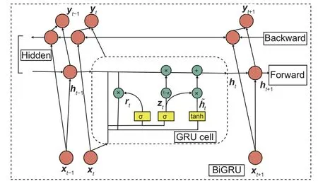
Fig.4 Structure of the BiGRU model

Step 3: construction of the spatial attention mechanism.The spatial attention mechanism is an adaptive spatial region selection mechanism,through which the BiGRU network is guided to pay more attention to the significant spatial regions on the grid graph.We take the number of passengers getting on and offthe grid as the weight.The input features are processed by MaxPool and AvgPool,then convoluted,and finally inputted to the Sigmoid function for activation,as defined in Eqs.(12) and (13).The process of building the spatial mechanism module is plotted in Fig.5.

Fig.5 Spatial attention mechanism

whereFis a characteristic graph,AvgPool represents average pooling,MaxPool denotes maximum pooling,fis the convolution operation,σ represents the Sigmoid activation function,andMsFdenotes the spatial attention parameter matrix.

3.4 Model implementation

In this work,the batch-size and epoch in the Bi-GRU structure are set as 4 and 180 respectively,and the numbers of neural network layers and neurons are 2 and 16 respectively.The process of EEMDNSABiGRU with Spark implementation is shown in Fig.6.

Fig.6 Implementation process of the EEMDNSABiGRU model

Step 1: data decomposition.The EEMD algorithm decomposes the 15-min interval passenger hotspot data in the grid to obtain a finite number of IMFs and a Res sequence.

Step 2: data normalization.Normalize the IMF and Res,and map them to a range of[0,1].

Step 3: model prediction.The normalized IMF and Res are inputted into the BiGRU model with spatial attention for prediction.

Step 4: result superposition.The prediction values are denormalized,and the values are summed to obtain the final prediction results.

4 Experiments

In this section,we validate the performance of the proposed EEMDN-SABiGRU model for passenger hotspot prediction with real-world taxi trajectory data from a case study.Specifically,the fit test is performed after EEMD and the original sequence.Then,the normalization test is executed on the sequence prediction results obtained from EEMD,and the effects before and after normalization are analyzed.Next,the prediction performances of 1-,10-,20-,and 30-day datasets in the 00-grid are compared using different models,and the results are analyzed in detail.Finally,the robustness of the EEMDN-SABiGRU model is evaluated with the 30-day dataset under different grids.

4.1 Experimental setup

The extensive experiments are performed on a Hadoop distributed platform with a Spark parallel computing framework.The experimental platform is configured with Hadoop 3.1.1+Spark 2.4.3 +Java+DL4J on Ubuntu 18.04 OS,AMD Ryzen7 4800H,and 8 GB ECC DDR3.

Moreover,the EEMDN-SABiGRU model is compared with LSTM,EMD-LSTM,EEMD-LSTM,GRU,EMD-GRU,EEMD-GRU,EMDN-GRU,CNN,and BP.

4.2 Experimental data

The experimental data come from the GPS trajectory data of 12 000 taxis in Beijing,China,in 2012,which have more than 9.0×108GPS trajectory records (about 50 GB).An example of the dataset is plotted in Fig.7.

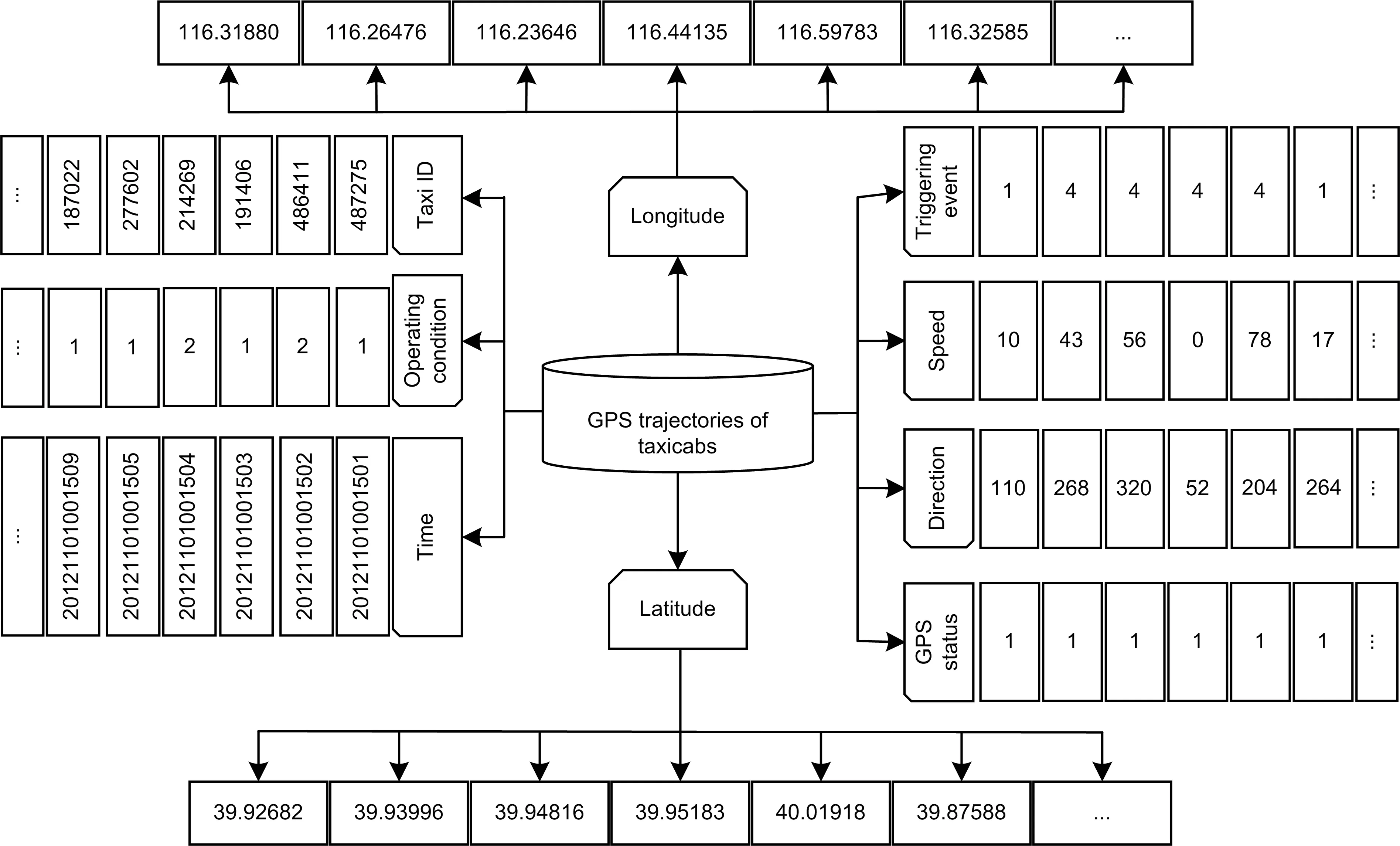
Fig.7 Taxi GPS trajectory data

Furthermore,to compare the effectiveness of the EEMDN-SABiGRU model,we divide the dataset into four groups (1-day: November 1;10-day:November 1-November 10;20-day: November 1-November 20;30-day: November 1-November 30),and the time interval of each group is 15 min.In addition,70%of the data are chosen as the training set,and 30%are used as the test set in all experiments.

4.3 Evaluation metrics

To validate the measures of effectiveness (MOEs) of the EEMDN-SABiGRU model,four metrics,mean absolute percentage error (MAPE),root mean square error (RMSE),mean absolute error (MAE),and maximum error (ME),are employed for evaluation:

whereXtis the real value of passenger hotspots,is the prediction value of passenger hotspots,andnis the total number of samples in the provided time.The MAPE value is used to compare the accuracy of each model.The lower the MAPE value,the higher the prediction accuracy.

4.4 Result analysis

4.4.1 Sequence prediction

EEMD is carried out with the 1-and 10-day datasets,and the decomposed series are tested for goodness-of-fit.The overall trend of the IMF1 series is steeper,because the original series are nonstationary series with significant differences.Next,the EEMD algorithm is repeated by subtracting the IMF1 series from the original series until no IMF series are generated.The 1-day dataset is shown in Fig.8a,and the results can be fitted perfectly with the original data.To further verify how well the sequences obtained by the EEMD algorithm fit the initial data,the amount of data is increased to 10-day and then the sequences are fitted to the original sequences,as plotted in Fig.8b.Obviously,the sum of the sequences fits the original dataset well,indicating that the EEMD algorithm does not produce missing data cases with the increased dataset.

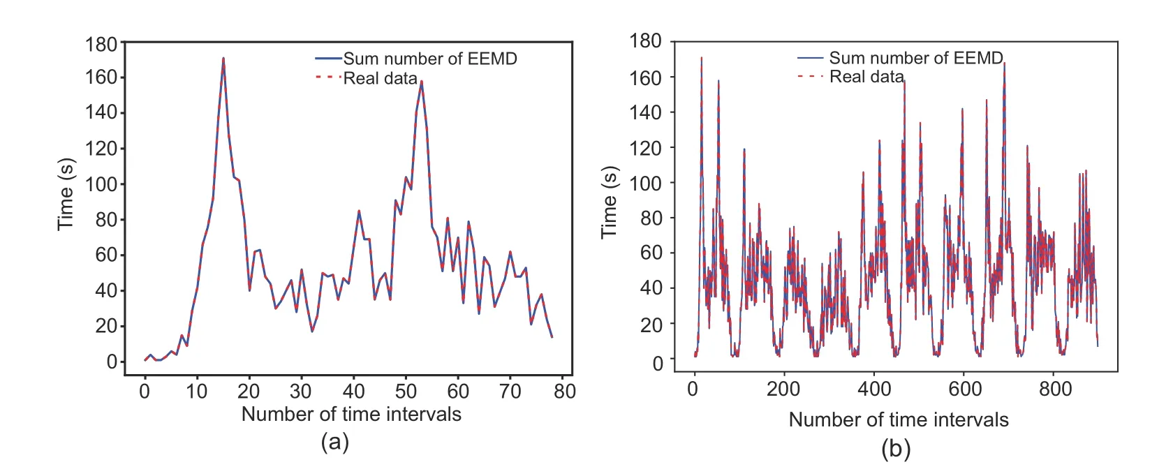
Fig.8 Data fit test of EEMD: (a) data test on the 1-day dataset;(b) data test on the 10-day dataset

4.4.2 Normalization test

Although the EEMD algorithm is suitable for dealing with non-smooth sequences and also solves the modal mixing problem of the EMD algorithm,there will be too many differences in values between IMF sequences during the decomposition process,which will cause BiGRU to fluctuate in prediction and lead to unsatisfactory overall prediction.We employ the normalization method to limit the preprocessed data to a specific range (e.g.,[0,1]or[-1,1]) and eliminate the adverse effects caused by singular sample data.Therefore,it is an excellent choice to normalize the EEMD sequences.The prediction results of the sequences before and after normalization are illustrated in Tables 1 and 2,respectively.

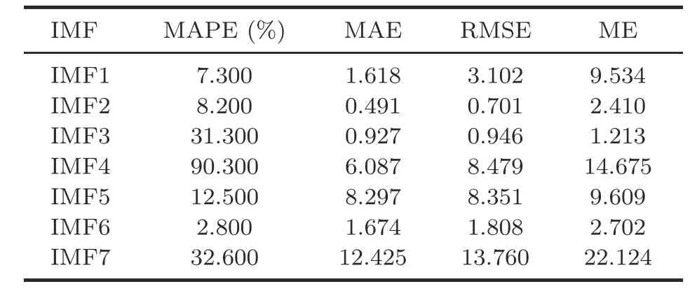
Table 1 Measures of effectiveness values of forecasting results before normalization

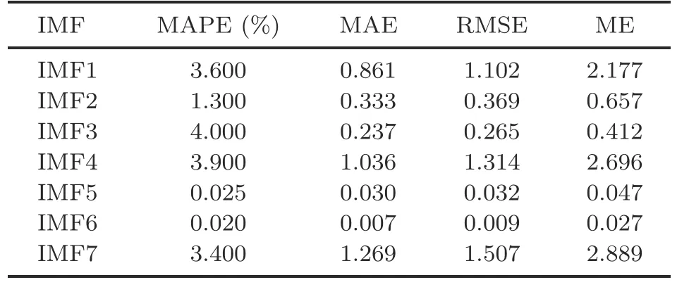
Table 2 Measures of effectiveness values of forecasting results after normalization

Tables 1 and 2 show that the normalized sequence prediction results are significantly superior to the pre-normalized sequence prediction results.Moreover,the prediction results before normalization compared with the sequence prediction results after normalization show a minimum reduction of 50.68% and a maximum reduction of 99.80% in MAPE,a minimum reduction of 32.18% and a maximum reduction of 99.64% in MAE,a minimum reduction of 47.36% and a maximum reduction of 99.62%in RMSE,and a minimum reduction of 66.03% and a maximum reduction of 99.51% in ME.Finally,combined with the above analysis,it is concluded that the results of sequence prediction are greatly improved after using the normalization method,so the EEMD algorithm is chosen to decompose and normalize the sequence for prediction.

4.4.3 Prediction results of different days in the 00-grid

We use a 00-grid with 1-,5-,10-,15-,20-,25-,and 30-day datasets from the road network for model validation,and compare EEMDN-SABiGRU with LSTM,EMD-LSTM,EEMD-LSTM,GRU,EMDGRU,EEMD-GRU,EMDN-GRU,CNN,and BP.

The MOE values of different models with seven datasets are shown in Table 3.We conduct finegrained analysis on four datasets: 1-,10-,20-,and 30-day.On the 1-day dataset,it is evident that the fit of the data with large fluctuations is greatly improved after using the EMD algorithm for data decomposition compared to the LSTM model,and the MOE values are greatly reduced.After using the EEMD algorithm,the MAE,RMSE,and ME values are increased,except for the reduced MAPE values,and all of them are lower than those of the LSTM model.Compared with the GRU model,the MOE values decrease significantly after using the EMD algorithm with the EEMD algorithm.Moreover,the prediction accuracy of the EEMD-GRU model is better than that of the EMD-GRU model.It can be concluded that the GRU model combined with the EEMD algorithm is significantly superior to the LSTM algorithm.Therefore,this work employs the GRU model combined with the EEMD algorithm for passenger hotspot prediction.As illustrated in Fig.S1j in the supplementary materials,the prediction values fit the real values well,and the evaluation metrics of EEMDN-SABiGRU are significantly lower than those of the comparable models.Among them,based on the 1-day dataset,compared with LSTM,EMD-LSTM,EEMD-LSTM,GRU,EMDGRU,EEMD-GRU,EMDN-GRU,CNN,and BP,the MAPE value of the EEMDN-SABiGRU model is reduced by 94.81%,87.50%,73.68%,94.09%,86.24%,81.48%,58.33%,95.21%,and 84.21%,respectively;MAE is reduced by 95.93%,66.50%,70.00%,95.28%,81.46%,72.30%,44.91%,95.08%,and 83.90%,respectively;RMSE is decreased by 96.85%,70.65%,81.68%,96.41%,84.52%,77.40%,55.04%,95.41%,and 84.98%,respectively;ME is decreased by 95.65%,67.33%,73.36%,95.25%,78.50%,64.90%,39.33%,91.71%,and 72.99%,respectively.Therefore,it can be concluded that the EEMDNSABiGRU model has better prediction performance on the 1-day dataset.

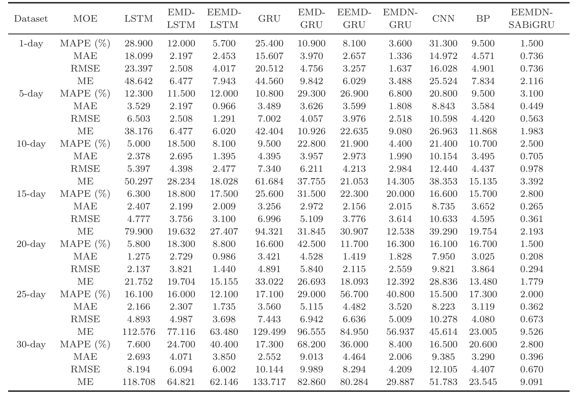
Table 3 Comparisons of models in different datasets using the 00-grid

On the 10-day dataset,from Fig.S2 in the supplementary materials,the LSTM,GRU,CNN,and BP models,although more effective in predicting data with relatively minor fluctuations,tend to decrease in accuracy once the fluctuations are large.With the addition of the EMD and EEMD algorithms,the MAPE values of the LSTM and GRU models increase,while the values of MAE,RMSE,and ME decrease.Although the predictions in high and low peaks tend to follow roughly the same trend as the test set,there are some numerical differences between the prediction values and the test set with the EMD-LSTM,EEMD-LSTM,EMD-GRU,and EEMD-GRU models.Moreover,the EMDNGRU and EEMDN-SABiGRU models fit the test set well after normalization.Therefore,in Table 3,the MOE values of EMDN-GRU and EEMD-GRU are lower than those of the other models.Finally,from Fig.S2j in the supplementary materials,it can be concluded that the EEMDN-SABiGRU model generates accurate predictions for both higher and lower volatility data compared to the LSTM,EMDLSTM,EEMD-LSTM,GRU,EMD-GRU,EEMDGRU,EMDN-GRU,CNN,and BP models.From Table 3,based on the 10-day dataset,compared with LSTM,EMD-LSTM,EEMD-LSTM,GRU,EMDGRU,EEMD-GRU,EMDN-GRU,CNN,and BP,MAPE is reduced by 50.00%,86.49%,69.14%,73.68%,89.04%,88.58%,43.18%,88.32%,and 76.64%,respectively;MAE is reduced by 70.35%,73.84%,49.46%,83.96%,82.18%,76.29%,64.57%,93.06%,and 79.83%,respectively;RMSE is decreased by 81.88%,77.76%,60.52%,86.68%,84.25%,76.79%,67.22%,92.14%,and 77.96%,respectively;ME is decreased by 93.26%,87.99%,81.18%,94.50%,91.02%,83.89%,76.29%,91.16%,and 77.59%,respectively.For passenger hotspot prediction on the 10-day dataset,the EEMDN-SABiGRU model can still obtain accurate prediction results.

As observed from Table 3,with the addition of the EMD and EEMD algorithms on the 20-day dataset,the MAPE,MAE,and RMSE values of the LSTM and GRU models increase,while the ME values decrease.When the EMD algorithm is replaced by the EEMD algorithm,all the MOE values are reduced,proving that the EEMD algorithm can compensate for the EMD algorithm’s modal mixing problem.Meanwhile,the MAPE values of the EEMD-LSTM and EEMDGRU algorithms are lower than those of the traditional LSTM and GRU,so we use the normalized EMDN-GRU algorithm to solve this problem.Finally,as shown in Table 3 and Fig.S3j in the supplementary materials,the EEMDN-SABiGRU model outperforms LSTM,EMD-LSTM,EEMDLSTM,GRU,EMD-GRU,EEMD-GRU,EMDNGRU,CNN,and BP.From Table 3,based on the 20-day dataset,compared with LSTM,EMDLSTM,EEMD-LSTM,GRU,EMD-GRU,EEMDGRU,EMDN-GRU,CNN,and BP,MAPE is reduced by 74.14%,91.80%,82.95%,90.96%,96.47%,87.18%,90.80%,90.68%,and 91.02%,respectively;MAE is reduced by 83.69%,92.38%,78.90%,93.92%,95.41%,85.34%,88.62%,97.38%,and 93.12%,respectively;RMSE is decreased by 86.24%,92.30%,79.58%,93.99%,94.96%,86.10%,88.51%,97.00%,and 92.39%,respectively;ME is decreased by 91.82%,90.97%,88.26%,94.61%,93.34%,90.17%,85.64%,93.83%,and 86.80%,respectively.The EEMDN-SABiGRU model is nevertheless able to obtain accurate passenger hotspot prediction results with the 20-day dataset.

With the 30-day dataset,it can be seen from Fig.S4 in the supplementary materials that the greater the fluctuation of the data,the worse the fit of the model,particularly the worst at the summit.The CNN,BP,LSTM,and GRU models have a worse fitting effect with real values when the data fluctuate significantly.The EMDN-GRU and EEMDNSABiGRU models also have excellent fitting results when the data fluctuate dramatically.Meanwhile,from Table 3,it is concluded that after the EMD and EEMD algorithms are used for LSTM and GRU,the RMSE and ME values gradually decrease.However,MAPE and MAE appear to increase because the increase in data leads to the difference between the values,resulting in unsatisfactory prediction results.In addition,the MAE,RMSE,and ME values of the normalized EMDN-GRU model decrease significantly,but the MAPE values are higher than those of the LSTM model due to the model’s lower ability to capture distinct features during training and prediction.However,the bi-directional gating mechanism of EEMDN-SABiGRU with the addition of spatial attention can solve these problems.Finally,from Fig.S4j in the supplementary materials,it can be concluded that the EEMDN-SABiGRU model outperforms LSTM,EMD-LSTM,EEMDLSTM,GRU,EMD-GRU,EEMD-GRU,EMDNGRU,CNN,and BP.From Table 3,based on the the 30-day dataset,compared with LSTM,EMDLSTM,EEMD-LSTM,GRU,EMD-GRU,EEMDGRU,EMDN-GRU,CNN,and BP,MAPE is reduced by 63.16%,88.66%,93.07%,83.82%,95.89%,92.22%,66.67%,83.03%,and 86.41%,respectively;MAE is decreased by 85.30%,90.27%,89.71%,84.48%,95.61%,91.13%,80.26%,95.78%,and 87.96%,respectively;RMSE is decreased by 91.82%,89.00%,88.84%,93.40%,93.29%,91.92%,84.08%,94.46%,and 84.80%,respectively;ME is decreased by 92.34%,85.98%,85.37%,93.20%,89.03%,88.68%,69.58%,82.44%,and 61.39%,respectively.The EEMDN-SABiGRU model obtains accurate prediction results for passenger hotspots on the 30-day dataset.

4.4.4 Prediction results of different grids

To further evaluate the scalability of the EEMDN-SABiGRU model,the surrounding grids,such as the 00-,55-,and 99-grid,are selected for prediction with the 30-day dataset,and the results are shown in Tables 4-6.

Table 4 shows the MOE values of the 00-,01-,10-,and 11-grid with the 30-day dataset.Table 5 illustrates the MOE values of the 55-grid peripheral grids 44,45,54,and 55 with the 30-day dataset.Table 6 shows the MOE values of the 99-grid peripheral grids 88,89,98,and 99 with the 30-day dataset.According to Tables 4-6,the average MAPE values of the EEMDN-SABiGRU model in the Spark framework are 3.150%,2.175%,and 2.275%,respectively,which indicates that the EEMDN-SABiGRU model is strongly reliable and scalable in predicting passenger hotspots between different grids in different areas,as illustrated in Fig.9.

Table 4 Measures of effectiveness for 00-grid with the same dataset

Table 5 Measures of effectiveness for 55-grid with the same dataset

Table 6 Measures of effectiveness for 99-grid with the same dataset

Fig.9 Comparisons of MOE values for EEMDN-SABiGRU under different grids with the 30-day dataset: (a)00-grid;(b) 55-grid;(c) 99-grid

4.4.5 Time complexity analysis

In this work,we compare the execution time of each model with 1-and 10-day datasets,as described in Table 7.

Table 7 Execution time of different models

From Table 7,the time complexity of the proposed EEMDN-SABiGRU model is in the same level as those of the other comparable models.Although our EEMDN-SABiGRU model does not improve the time complexity of passenger hotspot prediction,it has the same level of execution efficiency as other models.

In summary,the aforementioned prediction results demonstrate that the EEMDN-SABiGRU model shows excellent prediction performance.However,with the increased dataset,the value of ME increases,which shows that the prediction error of the model also increases.As shown in Fig.10,the prediction performances of the LSTM and GRU models after using EMD,EEMD,and EMDN are significantly improved with the 1-day dataset.With the 10-,20-,and 30-day datasets,after adding EMD and EEMD to the LSTM and GRU models,the RMSE and ME values decrease and the MAPE and MSE values increase,indicating that the neural network model incorporating the EMD and EEMD methods produces a decreasing trend of prediction performance when the dataset increases.The MOE values of the EEMDN-SABiGRU model fluctuate slightly with the 30-day dataset,which proves that the EEMDN-SABiGRU model generates excellent prediction stability when the prediction performance is satisfactory.In particular,the time complexity of the EEMDN-SABiGRU model is in the same level as those of the comparable models.

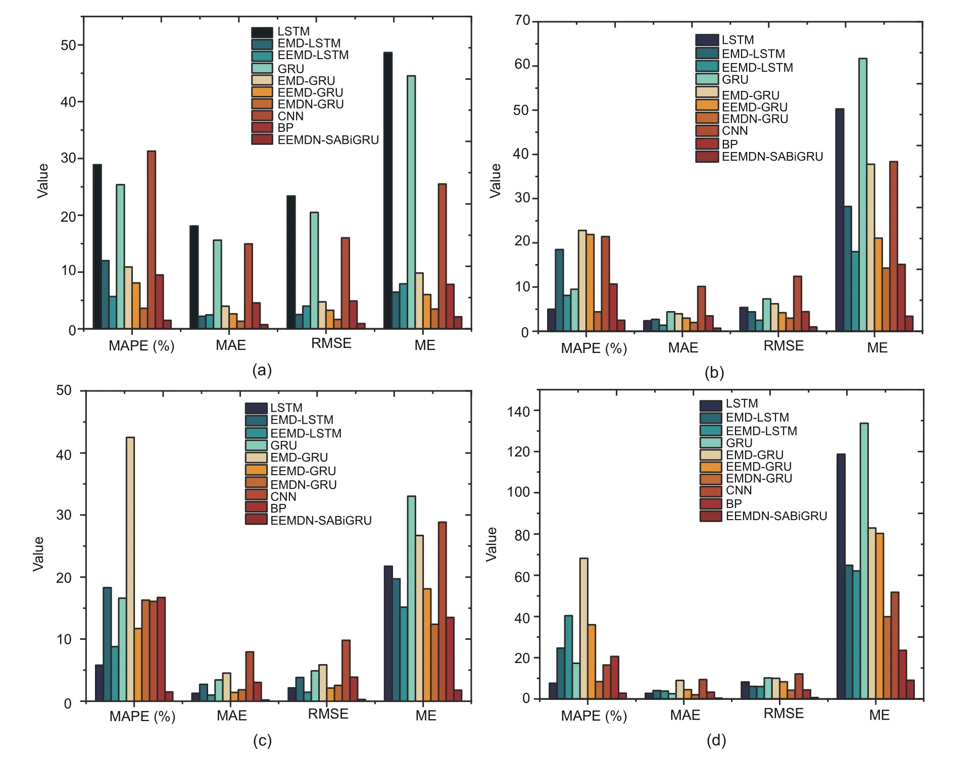
Fig.10 Comparisons of MOE values for different models with different datasets in the 00-grid: (a) 1-day;(b)10-day;(c) 20-day;(d) 30-day

5 Conclusions

This paper proposed a distributed EEMDNSABiGRU model on Spark to predict passenger hotspots.Specifically,the urban road network was rasterized under the Spark framework.Then,to improve the prediction accuracy of the model and to solve the non-smooth sequences and numerical differences,the EEMD algorithm and normalization method were introduced to process the rasterized road network data.Next,the fusion BiGRU model dealt with the deficiency that the GRU model cannot extract contextual information,and the spatial attention module was constructed to focus on the travel hotspot areas on the map and obtain the prediction results.Finally,the prediction results were merged by inverse normalization to obtain the final prediction results.In particular,the prediction results of the EEMDN-SABiGRU model were compared with those of the LSTM,GRU,EMD-LSTM,EMD-GRU,EEMD-LSTM,EEMD-GRU,EMDNGRU,CNN,and BP models.The experimental results demonstrated that EEMDN-SABiGRU is significantly superior to LSTM,GRU,EMD-LSTM,EMD-GRU,EEMD-LSTM,EEMD-GRU,EMDNGRU,CNN,and BP.From the experiment results,it can be concluded that the EEMDN-SABiGRU model can predict the passenger hotspots more accurately,and the prediction performance was still satisfactory with the increased dataset.

In future work,we will consider the effects of weather,traffic conditions,and passenger mobility on passenger hotspots,and validate the EEMDNSABiGRU model using GPS data from taxis in different cities.

Contributors

Dawen XIA and Jian GENG designed the research.Dawen XIA,Jian GENG,and Huaqing LI proposed the approaches and performed the experiments.Ruixi HUANG,Bingqi SHEN,and Yang HU processed the data.Dawen XIA,Jian GENG,and Huaqing LI drafted the paper.Dawen XIA,Jian GENG,Yang HU,Yantao LI,and Huaqing LI revised and finalized the paper.

Compliance with ethics guidelines

Dawen XIA,Jian GENG,Ruixi HUANG,Bingqi SHEN,Yang HU,Yantao LI,and Huaqing LI declare that they have no conflict of interest.

Data availability

The data that support the findings of this study are available from the corresponding authors upon reasonable request.

List of electronic supplementary materials

Fig.S1 Comparisons of models using the 1-day dataset

Fig.S2 Comparisons of models using the 10-day dataset

Fig.S3 Comparisons of models using the 20-day dataset

Fig.S4 Comparisons of models using the 30-day dataset