LDformer: a parallel neural network model for long-term power forecasting*
Ran TIAN,Xinmei LI,Zhongyu MA,Yanxing LIU,Jingxia WANG,Chu WANG
College of Computer Science &Engineering, Northwest Normal University, Lanzhou 730070, China
Abstract: Accurate long-term power forecasting is important in the decision-making operation of the power grid and power consumption management of customers to ensure the power system’s reliable power supply and the grid economy’s reliable operation.However,most time-series forecasting models do not perform well in dealing with long-time-series prediction tasks with a large amount of data.To address this challenge,we propose a parallel time-series prediction model called LDformer.First,we combine Informer with long short-term memory (LSTM) to obtain deep representation abilities in the time series.Then,we propose a parallel encoder module to improve the robustness of the model and combine convolutional layers with an attention mechanism to avoid value redundancy in the attention mechanism.Finally,we propose a probabilistic sparse (ProbSparse) self-attention mechanism combined with UniDrop to reduce the computational overhead and mitigate the risk of losing some key connections in the sequence.Experimental results on five datasets show that LDformer outperforms the state-of-the-art methods for most of the cases when handling the different long-time-series prediction tasks.
Key words: Long-term power forecasting;Long short-term memory (LSTM);UniDrop;Self-attention mechanism
1 Introduction
Power forecasting is an important part of power system planning and the basis of the economic operation of power systems.Accurate power forecasting helps provide a reliable decision-making basis for power system planning and operation,thus reducing power production costs (Ciechulski and Osowski,2021).Traditional prediction methods have achieved great results in meteorology,finance,industry,and transportation for short-term power forecasting problems.However,existing time-series methods still have limitations in long-time-series prediction:
1.Due to the highly complex and large-scale long-time-series data,traditional methods are limited in efficiently handling high-dimensional large data and representing complex functions (Han et al.,2021).It will forget some data and ignore the long-term dependency of the time-series data.
2.The model structure of traditional methods is not stable when long-term power forecasting is performed.
3.The existing attention mechanism is prone to losing key connections between sequences when capturing the dependencies among long-time-series data,leading to the degradation of prediction performance.
Aiming at the problem of long-time-series prediction,we propose LDformer,a parallel neural network model for long-term power forecasting based on the Informer framework (Zhou et al.,2021).The contributions of this study are summarized as follows:
1.We propose a parallel neural network model called LDformer,which combines the advantages of Informer and long short-term memory (LSTM) to effectively solve the problem of long-term power forecasting.Using LSTM to learn the long-term correlation of time-series data,the model has good long-term forecasting performance.
2.We propose a parallel encoder module that combines a convolutional layer and an attention mechanism to avoid value redundancy in the attention mechanism.Several experiments on different datasets validate the effectiveness and robustness of the parallel encoder and the convolutional layer.
3.We propose a probabilistic sparse (ProbSparse) self-attention mechanism combined with UniDrop.UniDrop does not need additional computational overhead or external resources.Combining UniDrop,Prob-Sparse attention mechanism can mitigate the risk of losing some key connections in the sequence.
2 Related works
Long-time-series prediction plays an essential role in decision-making in many fields,such as economy,transportation,medicine,hydrology,and energy (Zhang D et al.,2018;Chakraborty et al.,2019;Chuku et al.,2019;Xie and Lou,2019;Marcjasz et al.,2020).However,the prediction model may produce inaccurate results due to different patterns of the actual time series.In this paper,we analyze both machine learning and deep learning.
2.1 Machine learning
In time-series prediction,the Autoregressive Integrated Moving Average (ARIMA) model is widely used in various fields.Chen JF et al.(1995) developed an adaptive ARIMA model for short-term power forecasting of a power generation system.Viccione et al.(2020) applied the ARIMA model for tank water level prediction and analysis.Many researchers have also achieved better results by improving ARIMA models or combining ARIMA with other models.Xu et al.(2017) proposed an ARIMA and Kalman filterbased approach applied to road traffic real-time state prediction.Khan et al.(2020) proposed a waveletbased hybrid ARIMA model.However,although the ARIMA model has achieved great success in stable time-series prediction,there are no almost pure stationary data in the real-time-series data.Therefore,the application of the ARIMA model is limited by the data characteristics and is less general.As a result,many models other than ARIMA models have been applied to time-series forecasting.Syriopoulos et al.(2021) used a support vector machine (SVM) to predict shipping prices.Based on SVM,Ding et al.(2021) developed a time-series model based on the least squares support vector machine (LSSVM) and achieved better results.Nóbrega and Oliveira (2019) proposed sequential learning methods for the Kalman filter and a limited learning machine for regression and time-series prediction,obtaining better results.In addition to the normal case,many researchers have also modeled predictions for time-series data with outliers.Chen XY and Sun (2022) proposed a Bayesian time-factor decomposition framework for modeling and predicting multidimensional time series of specific spatiotemporal data in the presence of missing values.However,machine learning methods cannot obtain more accurate results for complex prediction problems.
2.2 Deep learning
With the development of deep learning,researchers have found that deep learning applies to complex time-series problems (Kim et al.,2018).Many scholars use convolutional neural networks (CNNs) to model and predict time-series data (Guo et al.,2019;Hosseini and Talebpour,2019).Cao and Wang (2019) applied CNN to stock forecasting.However,a CNN is more suitable for spatial correlation than time series.As a result,recurrent neural networks (RNNs) have emerged.Hu et al.(2020) applied RNNs to traffic flow prediction based on time-series analysis.Min et al.(2019) proposed an RNN-based intent inference model to solve the time-series prediction problem.Many studies have proven that RNNs have obvious advantages in time-series prediction (Xiao et al.,2019;Zhang L et al.,2019).However,when the time-series is too long,the problems of gradient disappearance and gradient explosion may occur in RNN training (Zheng and Huang,2020).
Karevan and Suykens (2020) proposed LSTM to solve these problems.LSTM is more suitable for long-time-series than RNN.Therefore,many deep learning models based on LSTM are applied to timeseries prediction.Zhang TJ et al.(2019) used LSTM for gas concentration prediction.Miao et al.(2020) proposed a novel LSTM framework for short-term fog prediction,consisting of an LSTM and a fully connected layer.Their experiments showed that the framework outperformed K-nearest neighbor (KNN),Ada-Boost,and CNN algorithms.Gai et al.(2021) proposed a new parking space prediction model based on LSTM,providing a more accurate prediction.Many researchers have also proposed a combined model of LSTM and other models (Ran et al.,2019;Wang ZP et al.,2020),which proves the feasibility of LSTM in time-series prediction.However,we can learn from Khandelwal et al.(2018) that the adequate context size of the language model using LSTM is approximately 200 tokens on average.Nevertheless,the model can only distinguish 50 tokens in the vicinity,which indicates that even LSTM has difficulty capturing longterm dependencies.
In recent years,the transformer has been applied to many fields to perform long-time-series prediction tasks.Wu N et al.(2020) applied the transformer model to the prediction of influenza-like diseases,and this method can learn complex patterns and dynamics from time-series data using the self-attention mechanism.As a general framework,the transformer can not only be applied to univariate and multivariate time-series data,but can also be used for time-series embedding.However,because the point-by-point dot product in the transformer architecture is insensitive to the local context,its spatial complexity is too large.Therefore,Li et al.(2019) proposed the LogSparse transformer,which improves the prediction accuracy of time series with fine granularity and strong long-term dependence under a limited memory budget.Zhou et al.(2021) proposed the Informer and applied it to electricity consumption planning.Unlike the selfattention mechanism used in the transformer (Vaswani et al.,2017),this model proposes a new ProbSparse self-attention (Zhou et al.,2021),which minimizes the complexity and improves the transformer model’s calculation,memory,and efficiency.Although the existing time-series prediction methods have promoted the development of the time-series field to a certain extent,there is still room for improvement.Because of the increase in data volume,many time-series prediction models overlook deep representation abilities of temporal data,and also have problems such as numerous parameters,large memory consumption,and long operation time.
Compared with previous work,LDformer not only considers the deep representation of temporal data,but also mitigates the risk of losing critical connections between sequences while ensuring minimum complexity.In addition,LDformer combines the convolutional layer and the attention mechanism to obtain a parallel encoder module,which prevents redundancy in the attention mechanism while improving model robustness.These methods effectively improve the prediction accuracy.
3 Preliminaries
As shown in Eq.(1),the objective of long-term power forecasting is to use modelfto predict the power load data of a certain data point atntime steps based on historical power load data from multiple data points atmtime steps.
4 Long-time-series prediction model
The overall framework of LDformer is as shown in Fig.1.LDformer contains LSTM,encoder,and decoder structures.First,the time-series data enter the embedding layer,at which data,location,and time information is converted into a uniform dimension and then merged.The processed data then enter the LSTM,allowing for more effective use of long-term temporal information.Second,the data enter the encoder,which uses a multichannel parallel mode to improve model robustness to receive long-sequence inputs.At the same time,we extract the main features by adding convolution layers in the encoder module,and the convolution layer can generate a concentrated attention feature map to reduce feature redundancy.The decoder receives long-sequence inputs and predicts the output element immediately in the form of generation.After the embedding layer,the data enter the decoder.To ensure that the output decoded at timetdepends only on the output before timet,X0is a placeholder for the target sequence,padded with 0.A mask is added to the first attention of the decoder to prevent the target information from being used earlier.Finally,the prediction results of the last column are outputted through a fully connected layer.
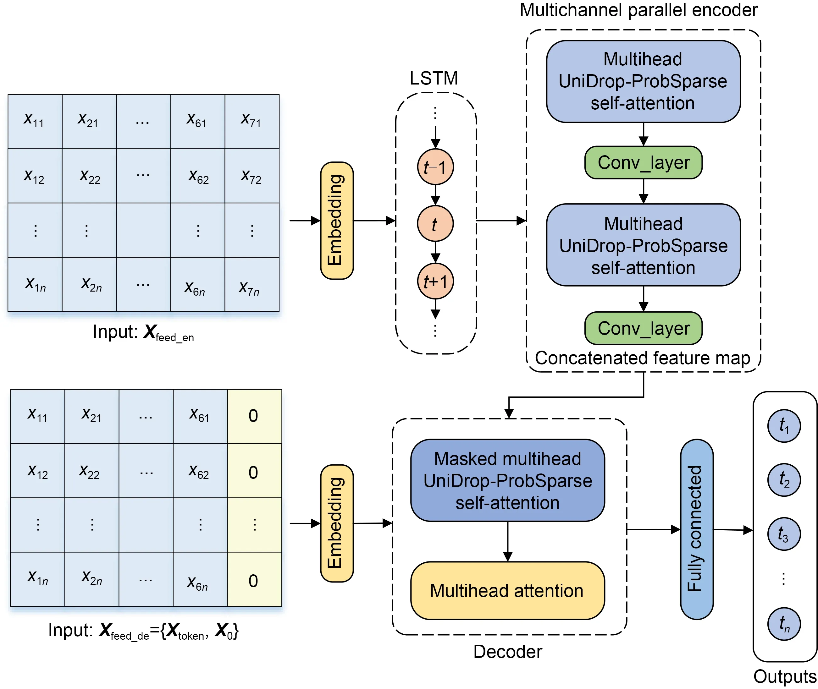
Fig.1 Framework of LDformer
4.1 Embedding layers with multiple perspectives
First,the preprocessed data are unified into the same dimension through data encoding,position encoding,and timestamp encoding,and then the final embedding result is obtained by summing the results of these three encodings.
1.Data embedding (DE): Convert data dimensionxinto uniform dimensiondmodelusing one-dimensional (1D) convolution.The formula is as follows:
2.Position embedding (PE) (Vaswani et al.,2017):Compared to RNNs,positional embedding uses a different approach where elements within the input sequence are processed concurrently,thereby preserving the positional information of each element within the sequence.Although the processing speed of RNN is higher than that of PE,it ignores the order of elements in the sequence,so we choose positional embedding.The formulae are as follows:
where pos denotes the position of the element in the sequence,dmodeldenotes the dimension of the element vector,andidenotes the position of the element vector.
3.Time embedding: There are various methods for time embedding: month_embed,day_embed,weekday_embed,hour_embed,and minute_embed.The time slice of the dataset used in this paper is mainly in hours and minutes,so hour_embed and minute_embed are chosen to obtain the timestamp encoding results.
The sum of these three embedding components is the output of the final embedding layer.The overall embedding layer structure is shown in Fig.2.
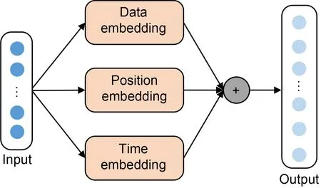
Fig.2 Embedding layer structure
The data outputted by embedding are sent to LSTM for feature extraction.For not affecting the input of the subsequent encoder,this study makes the output of LSTM consistent with the output of embedding;i.e.,the LSTM output dimension remains asdmodel.The output of LSTM is the input of the encoder.LSTM can perform better in long sequences.Therefore,using LSTM can extract deep representation abilities in the time series and improve the prediction accuracy.
4.2 Multichannel parallel encoder module
We build the encoder module by combining the attention mechanism with the convolutional layer.It takes four channels of lengthL,L/2,L/4,andL/8,and executes them in parallel.The convolutional layer performs dimensional pruning and reduces the memory footprint before the output of the upper layer is sent to the lower layer of the multihead attention module.The convolutional layer has one fewer layer than the encoder.The multichannel parallel encoder module is shown in Fig.3.
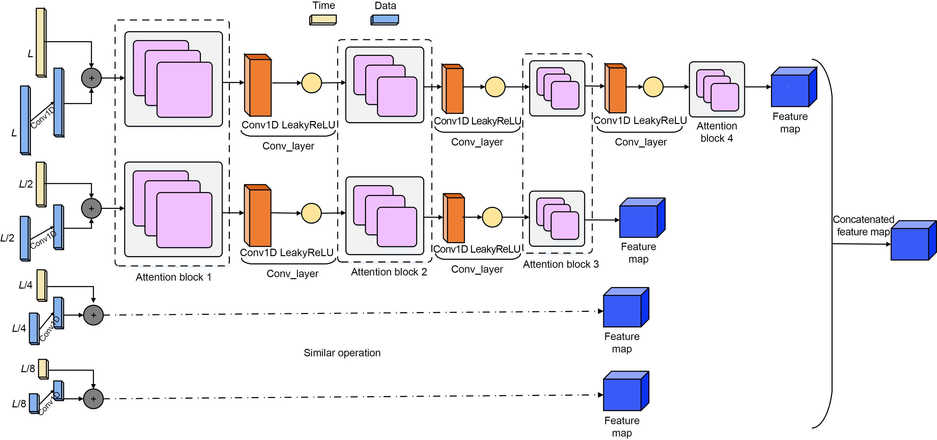
Fig.3 Multichannel parallel encoder module (References to color refer to the online version of this figure)
The encoder is used mainly to extract robust remote dependencies from time-series data.The overall architecture of the encoder is roughly the same as that of the transformer.It includes mainly two sublayers,the multihead attention layer (ProbSparse selfattention mechanism combined with UniDrop) and the feed-forward layer composed of two linear mappings.A batch normalization layer follows both sublayers,with jump connections between the sublayers.
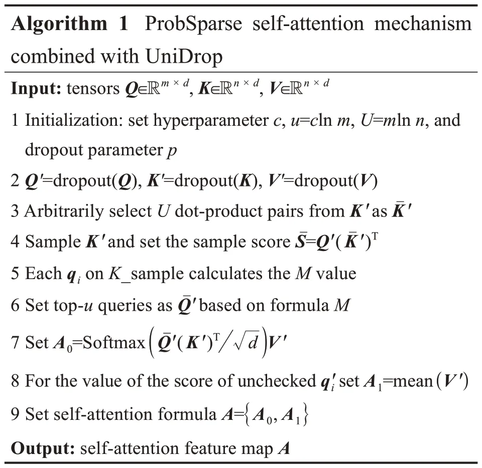
4.2.1 ProbSparse self-attention mechanism combined with UniDrop
ProbSparse self-attention mechanism may create some risk of critical connection loss.To address this problem,we propose a ProbSparse self-attention mechanism combined with UniDrop.Unlike the self-attention mechanism and ProbSparse self-attention mechanism,we consider other possible problems while retaining their advantages.
The canonical self-attention mechanism consists of a query and a set of key-value pairs.The formula is as follows (Vaswani et al.,2017):
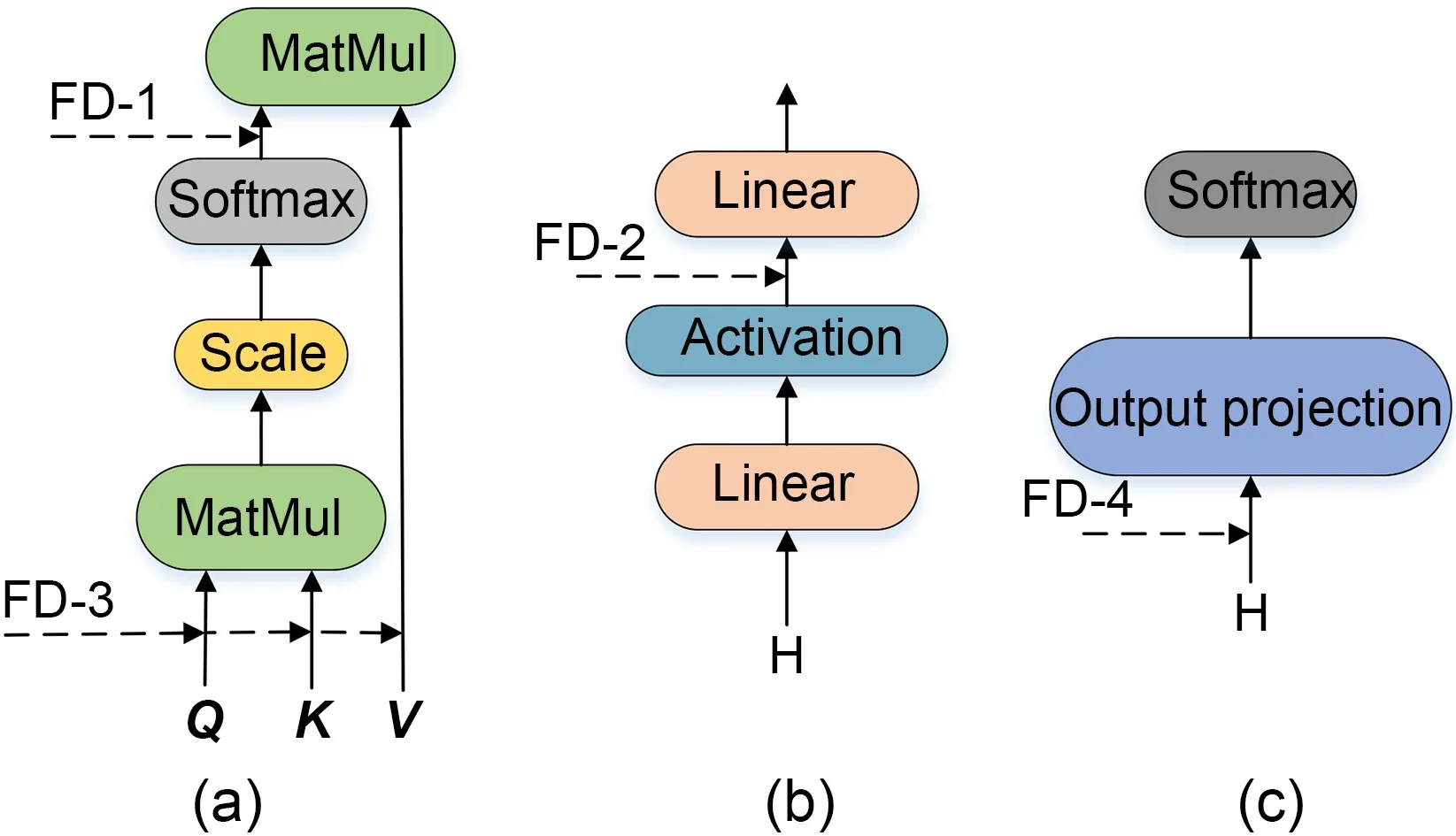
Fig.4 UniDrop structure: (a) attention;(b) feed forward;(c) output prediction (MatMul: matrix multiplication;H:hidden layer)
Define the attention of theithrow,ofQ',K',V'obtained after dropout as a kernel smoother in the form of probability:
Dropping the constant,the sparsity measure of theithquery can be defined as
Eq.(9) traverses all queries that require the computation of each dot-product pair,but the log-sum-exp (LSE) operation may have numerical stability issues.Based on this,the above formula is improved to obtain the final sparsity measure formula:
Based on the above steps,we obtain ProbSparse self-attention combined with UniDrop by allowing each key to pay attention to onlyudominant queries:
4.2.2 Convolutional layer
As a natural consequence of the ProbSparse attention mechanism combined with UniDrop,the feature mapping of the encoder produces a redundant combination of valuesV'.In the next layer,we use convolution to extract dominant features for processing so that they generate a focused attentional feature map,as shown in Fig.3,which will largely reduce the temporal dimension of the input.CNN is good at identifying simple patterns in data and generating complex patterns in more advanced layers.Conv1D is effective in obtaining features of interest from data whose locations are not highly correlated,and Conv1D can be well applied to time-series analysis of sensor data.Therefore,we select Conv1D to extract features and set its convolution kernel as 3×3.The formula is as follows:
where [·]ABcontains the basic operations in the multihead attention and attention block,and Conv1D uses the LeakyReLU activation function to execute in the time dimension.LeakyReLU is a variant of ReLU.It introduces some changes when the input value is less than 0,alleviates the sparsity of ReLU,and inherits the advantages of ReLU.It can also speed up the convergence,alleviate the gradient disappearance and explosion problems,and simplify the calculation.The LeakyReLU activation function is as follows:
4.3 Decoder
The decoder generates the time-series output by a forward process,and part of its structure can be referred to as the decoder structure in the transformer,as shown in Fig.5.
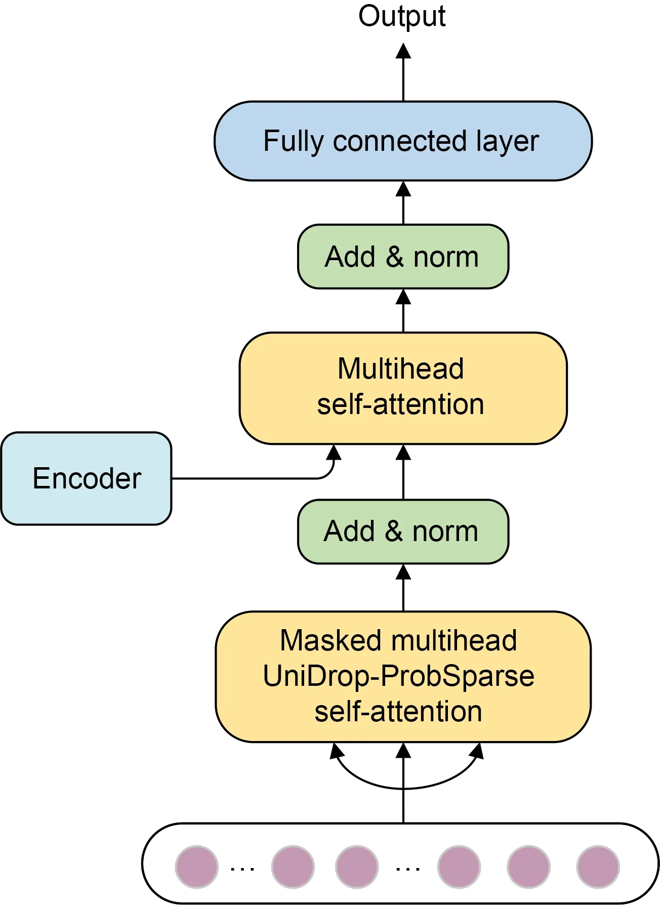
Fig.5 Decoder for growing sequence output through forward process generation
The decoder consists of two layers of attention mechanism and a linear mapping feed-forward layer.The decoder’s input vector is as follows:
The first layer of attention is the ProbSparse selfattention mechanism combined with UniDrop,as shown in Eq.(11).We set the masked multihead self-attention to -∞.It prevents focusing on the future position in the training process to avoid the autoregression problem.The second layer of attention is ordinary selfattention,as shown in Eq.(5).An add &norm layer follows both layers of attention.Add &norm is calculated as follows:
Finally,the prediction results are outputted directly through a fully connected layer.
5 Experiments and analyses
5.1 Datasets
We extensively perform experiments on five datasets,namely,the ETTm1,ETTh1,ETTh2,PEMS03,and weather datasets.ETTm1,ETTh1,and ETTh2 are collectively referred to as the ETT dataset.Table 1 shows the description of the datasets.

Table 1 Datasets and prediction task descriptions
ETT (Zhou et al.,2021): ETT is a key indicator of the long-term deployment of electricity.Here are two years of data collected from two cities in China.ETTm1 takes one data point every 15 min.ETTh1 and ETTh2 take one data point every hour.Each data point consists of the target value oil temperature (OT) and six different types of external load values,i.e.,high useful load (HUFL),high useless load (HULL),middle useful load (MUFL),middle useless load (MULL),low useful load (LUFL),and low useless load (LULL).We use a multivariate prediction univariate model with six power load features to predict the target value OT.According to the time characteristics,we divide the training set,validation set,and test set by 12,4,and 4 months,respectively.
Weather (Zhou et al.,2021): This dataset contains local climate data for nearly 1600 U.S.locations.Each data point consists of a target value wet bulb and 11 climate features.We divide the training set,validation set,and test set by 12,4,and 4 months,respectively.
PEMS03 (Wang C et al.,2023): This dataset is the traffic flow data of the California highway network.It is divided into five-minute intervals and contains data from 307 sensors for three months from 2018/9/1 to 2018/11/30.This experiment captures three months of traffic data from the first seven sensors.The dataset is divided by 7:2:1 into a training set,test set,and validation set.The seventh sensor is used as the target sensor for the experiment.
5.2 Experimental setting
In this study,the model uses both parallel and nonparallel modes in the encoder.The parallel mode has four channels executing in parallel and three stacks.The decoder contains two stacks.The sampling factorcin the top-uformula is set to 5.The parameter in dropout is 0.1.The number of multihead attentionn-heads is set to 8.When predicting the target sequence,the mean square error (MSE) is selected as the loss function,and the whole model is returned from the output of the decoder.The learning rate in the experimental setup decreases from 1e-04 and decays by a factor of 2 for each period.The model employs the Adam optimizer as its optimization algorithm,with 10 epochs and a batch size of 64.Moreover,prior to conducting the experiment,each input dataset is subjected to a standardization procedure.
Assessment metrics: three evaluation indexes,MSE,mean absolute error (MAE),and root mean square error (RMSE),are used.The primary reason for choosing RMSE is that,compared to MSE and other evaluation metrics,RMSE has advantages such as greater intuitiveness,stronger robustness,and easier interpretability in the assessment of model performance.Consequently,RMSE is widely adopted in numerous practical applications.For example,when RMSE is equal to 10,the regression effect can be considered to differ by 10 on average compared to the true value.The indicator equations are as follows:
whereyis the true value andis the prediction value.
5.3 Experimental results and analyses
We conduct comparative experiments on five datasets and multiple prediction tasks,comparing widely used RNN,LSTM,and gated recurrent unit (GRU) commonly employed in long-time-series prediction,as well as the representative Informer algorithm and its Informer (np) model under nonparallel conditions,with our parallel model LDformer and nonparallel LDformer (np).The specific description of the datasets is shown in Table 1.The corresponding experimental results are shown in Tables 2-5.
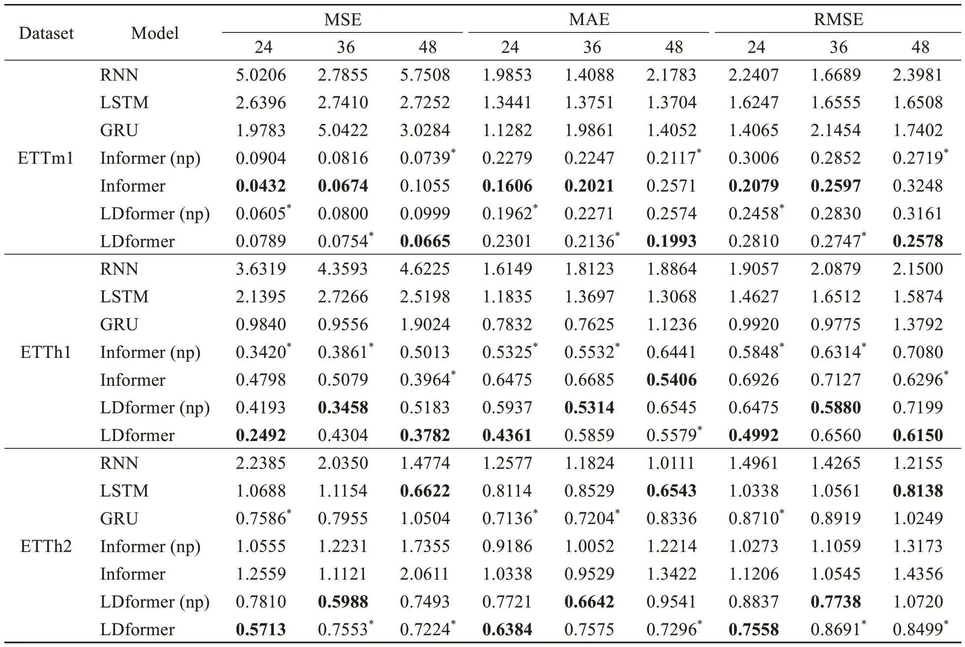
Table 2 Performance comparison of short-time-series prediction tasks in the ETT dataset at different prediction lengths (24,36,48)
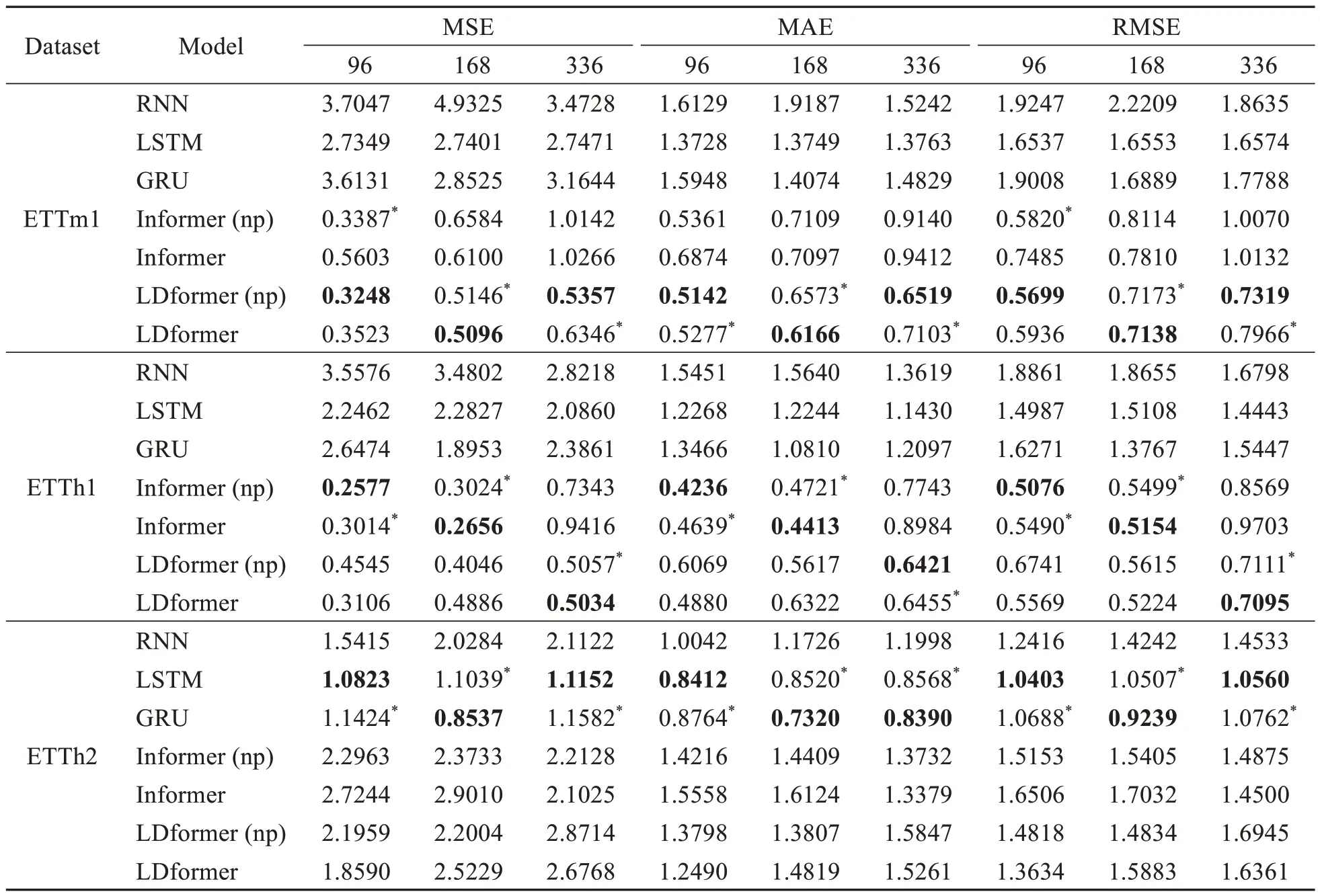
Table 3 Performance comparison of long-time-series prediction tasks in the ETT dataset at different prediction lengths (96,168,336)
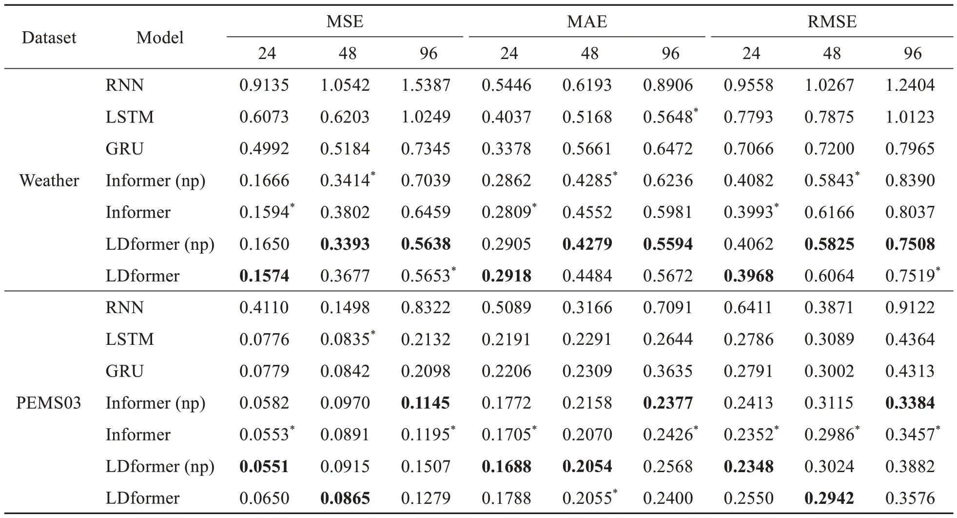
Table 4 Performance comparison of short-time-series prediction tasks in the weather and PEMS03 datasets at different prediction lengths (24,48,96)

Table 5 Performance comparison of long-time-series prediction tasks in the weather dataset at prediction lengths of 168,336,and 720 and the PEMS03 dataset at prediction lengths of 288,336,and 720
Tables 2 and 3 show the prediction performance of the baseline models and our models for short-and long-time-series of the ETT dataset,respectively.As the prediction length increases,the prediction performance of LDformer continues to increase in all datasets.This demonstrates the success of LDformer in improving prediction performance in solving long-time-series prediction problems.In the ETTm1 dataset,when the prediction length is 48,MSE,MAE,and RMSE of the LDformer model proposed in this paper are 37.0%,22.5%,and 20.6% lower than those of Informer,respectively.As the prediction length increases,the advantages of the LDformer become more apparent.When the prediction length is 168,MSE,MAE,and RMSE of LDformer are reduced by 16.5%,13.1%,and 8.6% compared to those of Informer,respectively.When the prediction length is 336 in the ETTm1 dataset,the LDformer (np) model has the optimal result,while the LDformer model shows the suboptimal result.
When the prediction length in ETTh1 is 24,MSE,MAE,and RMSE of LDformer are 74.7%,44.3%,and 49.7% lower than those of the traditional GRU model,respectively.After increasing the prediction length,Informer shows good performance for the ETTh1 dataset when the prediction length is 96 and 168.However,the performance of LDformer is better than those of traditional models in most cases.In the ETTh2 dataset of long-time-series prediction,the model in this paper outperforms traditional models.This phenomenon may be caused by the anisotropy of the feature dimensions.It is beyond the scope of this paper,and we will explore it in the future work.ETTh2 contains a large amount of continuous null data.
Tables 4 and 5 show the prediction performance of the baseline models and the models proposed in this paper for short-and long-time-series in the weather and PEMS03 datasets,respectively.For the weather dataset,when the prediction length is 168,MSE,MAE,and RMSE of LDformer are reduced by 29.4%,14.4%,and 16.0%,respectively,compared to those of Informer (np).For the PEMS03 dataset,when the prediction length is 336,MSE,MAE,and RMSE of LDformer are reduced by 12.6%,9.8%,and 6.5%,respectively,compared to those of Informer.The experiments show that the models proposed in this paper achieve better results for the PEMS03 dataset with a time interval of 5 min and the ETTm1 dataset with a time interval of 15 min.
LDformer accurately obtains the temporal information of each feature,where LSTM learns the longterm dependency of temporal data and fully exploits deep representation abilities among time-series data.The ProbSparse attention mechanism combined with UniDrop inherits the advantages of the ProbSparse attention mechanism,while avoiding the attention mechanism losing some key connections in the sequence when considering data correlation.Meanwhile,the encoder module adopts a multichannel parallel model to improve the robustness of LDformer.
We calculate the average error between the true and prediction values for different datasets.The error is plotted as a histogram,as shown in Figs.6 and 7.
In the short-time-series prediction (Fig.6),LDformer has the smallest average error between the prediction and true values,and the prediction accuracy is higher than that of other models.For long-time-series prediction (Fig.7),LDformer still achieves good results.However,the results are unsatisfactory due to the availability of null data in the ETTh2 dataset.LDformer combines the advantages of Informer and LSTM,and uses four channels in the encoder to improve the stability of the model.It also uses Prob-Sparse self-attention combined with UniDrop to reduce the loss of some key connections in the sequence and improves the accuracy of long-time-series prediction.
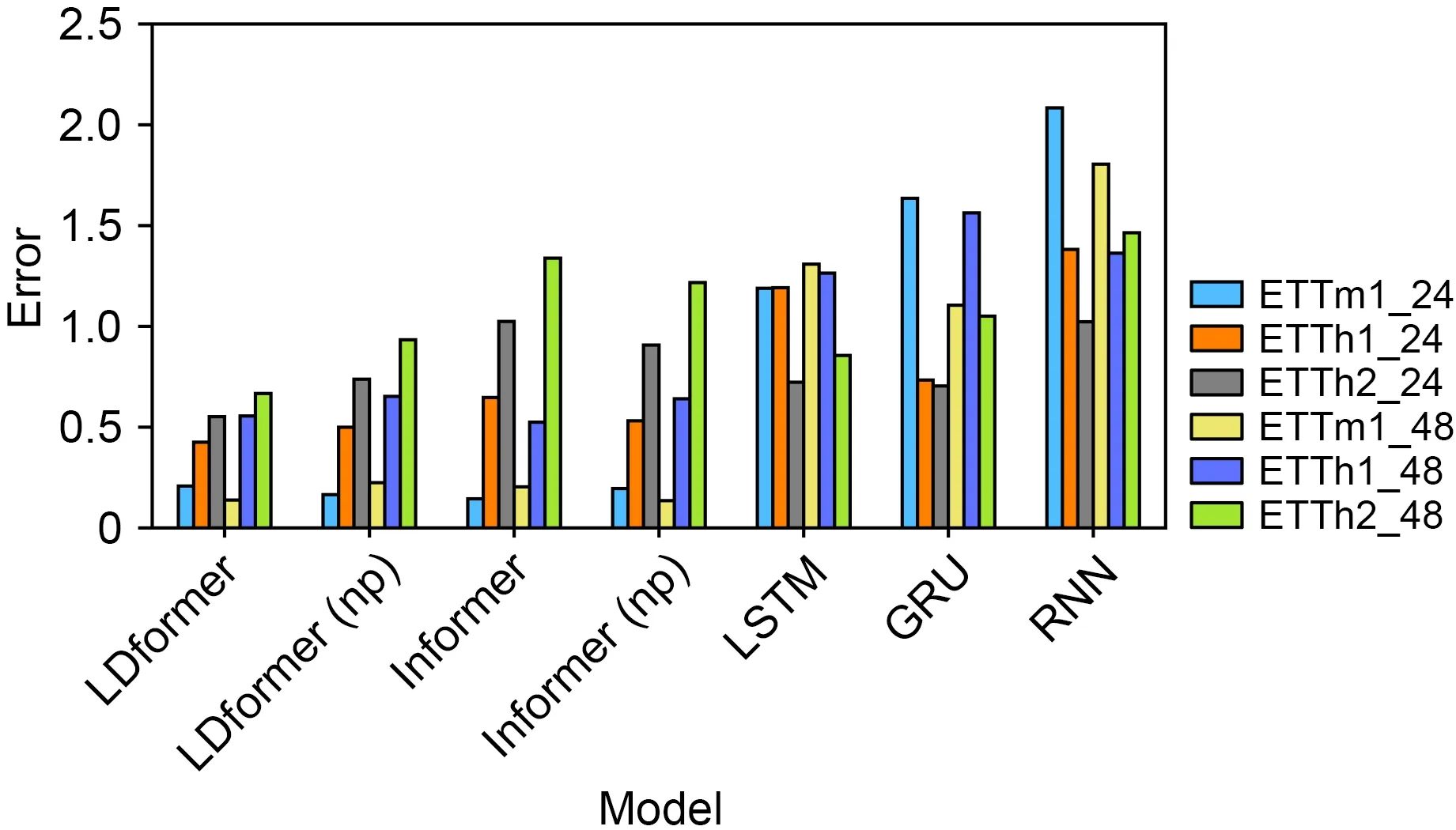
Fig.6 Average error of the true and prediction values in the short-time-series prediction (References to color refer to the online version of this figure)
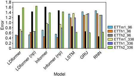
Fig.7 Average error of the true and prediction values in the long-time-series prediction (References to color refer to the online version of this figure)
We plot the average loss corresponding to different learning rates in the four models.As shown in Fig.8,the LDformer (np) proposed in this paper converges faster than the LDformer model.
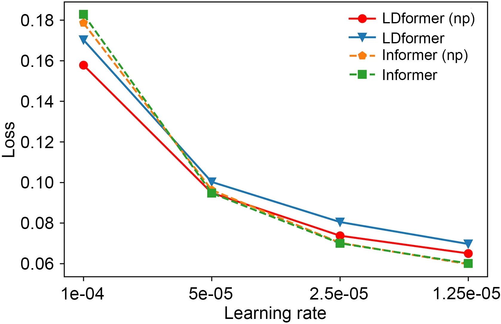
Fig.8 Convergence of loss with a decreasing learning rate for the ETTh1 dataset at a prediction length of 24
Fig.9 shows the training runtime profiles of several models with an increasing number of epochs.Under the early stop mechanism,both LDformer and LDformer (np) stop training at the fourth epoch,Informer stops training at the fifth epoch,and Infomer (np) stops training at the sixth epoch.Informer (np) obtains the optimal result at the sixth epoch.The training time of the models in this paper is significantly less than that of other models.Our proposed ProbSparse attention mechanism combined with UniDrop reduces the number of parameters without increasing the time complexity.Convolutional layers extract dominant features,reducing the temporal feature dimension and avoiding redundancy in the attention mechanism.This is the key factor that reduces the training time.
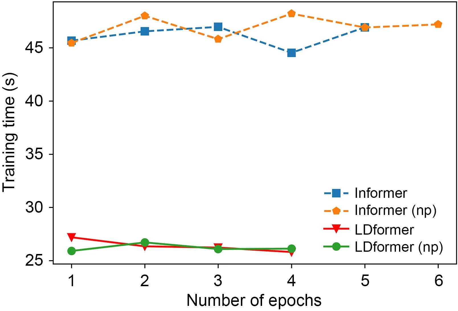
Fig.9 Training time comparison
We perform ablation experiments for each innovation point to further evaluate the effectiveness of the individual components in LDformer.Table 6 shows several models with various innovation points removed.

Table 6 Introduction to the ablation experiment modules
We compare the MSE and MAE of our models on the four prediction tasks with those of the models without innovation point.Table 7 shows that the cancellation of each innovation point affects the results.Through LSTM,LDformer can extract deep representation abilities from time-series data.This is achieved by the use of LSTM memory cells and gate mechanisms.Through LSTM memory cells and gate mechanisms,LSTM can effectively capture long-term dependencies and longer contextual information.UniDrop reduces the number of parameters and computational complexity,improving the model’s parallel computing capabilities.Multiple parallel channels contribute to a more stable model structure,by accepting various long sequences,which increases the model’s robustness to input noise and variations,making it more adaptable to different input conditions and data distributions.The convolutional layer reduces the potential complexity and computational cost of the attention mechanism by reducing the number of parameters.By combining these modules,LDformer achieves optimal results on most prediction tasks.
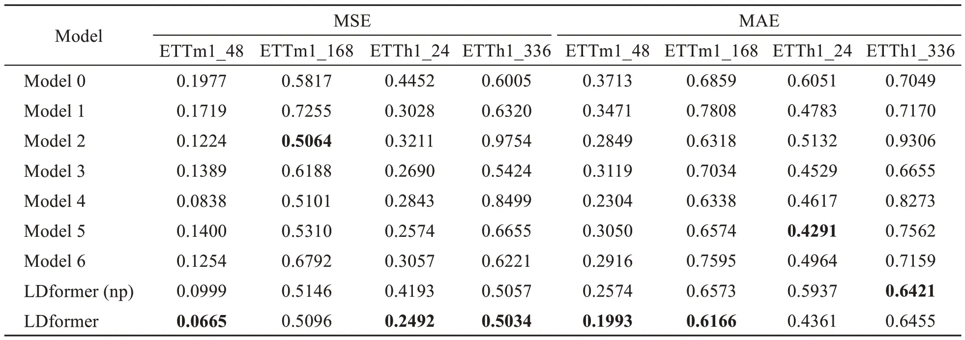
Table 7 The MSE and MAE of different models for the ETTm1 dataset at prediction lengths of 48 and 168 and the ETTh1 dataset at prediction lengths of 24 and 336
6 Conclusions
In this paper,we propose a long-term power forecasting model LDformer and its nonparallel state LDformer (np) to solve the long-time-series prediction problem with the power dataset ETT as an example.The LDformer model is useful for obtaining more accurate prediction results without increasing the time complexity.First,ProbSparse self-attention mechanism combined with UniDrop is proposed to replace ProbSparse self-attention mechanism,effectively avoiding the risk of losing key connections between sequences without increasing the complexity.Second,two perspectives,parallel and nonparallel,are used in the encoder module for comparison.Considering the number of parameters and model stability,we use convolutional layers for data extraction between attention modules.Finally,we combine the improved model with LSTM to capture the long-range time-series information and extract deep representation abilities in the time series to improve prediction accuracy.Experimental results confirm that LDformer performs better on long-time-series prediction tasks for short-interval datasets.For each innovation point proposed in this study,ablation experiments have been conducted to demonstrate the innovation points’ feasibility.However,the method presented in this study still has potential for improvement in dealing with long-term-series prediction tasks for long-interval datasets.
Contributors
Ran TIAN designed the research.Xinmei LI developed the methodology,curated the data,and worked on the software.Zhongyu MA conducted the investigation.Yanxing LIU processed the data.Jingxia WANG conducted the data visualization and result validation.Chu WANG verified the experimental results.Xinmei LI drafted the paper.Ran TIAN revised and finalized the paper.
Compliance with ethics guidelines
Ran TIAN,Xinmei LI,Zhongyu MA,Yanxing LIU,Jingxia WANG,and Chu WANG declare that they have no conflict of interest.
Data availability
The data that support the findings of this study are available from the corresponding author upon reasonable request.
 Frontiers of Information Technology & Electronic Engineering2023年9期
- Frontiers of Information Technology & Electronic Engineering的其它文章
- Matrix-valued distributed stochastic optimization with constraints∗
- Distributed optimization based on improved push-sum framework for optimization problem with multiple local constraints and its application in smart grid∗
- A home energy management approach using decoupling value and policy in reinforcement learning∗
- Exploring nonlinear spatiotemporal effects for personalized next point-of-interest recommendation
- Mixture test strategy optimization for analog systems∗#
- A distributed EEMDN-SABiGRU model on Spark for passenger hotspot prediction∗#
