Parameter sensitivity analysis for a biochemically-based photosynthesis model

Tuo Han, Qi Feng, TengFei Yu

Key Laboratory of Eco-Hydrology of Inland River Basin, Northwest Institute of Eco-Environment and Resources, Chinese Academy of Sciences (CAS), Lanzhou, Gansu 730000, China

Keywords: Sobol’ method Morris method Photosynthesis Parameters sensitivity analysis FvCB model

ABSTRACT A challenge for the development of Land Surface Models(LSMs)is improving transpiration of water exchange and photosynthesis of carbon exchange between terrestrial plants and the atmosphere,both of which are governed by stoma in leaves.In the photosynthesis module of these LSMs, variations of parameters arising from diversity in plant functional types (PFTs) and climate remain unclear.Identifying sensitive parameters among all photosynthetic parameters before parameter estimation can not only reduce operation cost,but also improve the usability of photosynthesis models worldwide.Here, we analyzed 13 parameters of a biochemically-based photosynthesis model (FvCB), implemented in many LSMs, using two sensitivity analysis (SA) methods (i.e., the Sobol’ method and the Morris method) for setting up the parameter ensemble.Three different model performance metrics, i.e.,Root Mean Squared Error (RMSE), Nash Sutcliffe efficiency (NSE), and Standard Deviation (STDEV) were introduced for model assessment and sensitive parameters identification.The results showed that among all photosynthetic parameters only a small portion of parameters were sensitive, and the sensitive parameters were different across plant functional types: maximum rate of Rubisco activity (Vcmax25), maximum electron transport rate (Jmax25), triose phosphate use rate (TPU) and dark respiration in light (Rd) were sensitive in broad leafevergreen trees (BET), broad leaf-deciduous trees (BDT) and needle leaf-evergreen trees (NET), while only Vcmax25 and TPU are sensitive in short vegetation (SV), dwarf trees and shrubs (DTS), and agriculture and grassland(AG).The two sensitivity analysis methods suggested a strong SA coherence;in contrast,different model performance metrics led to different SA results.This misfit suggests that more accurate values of sensitive parameters,specifically,species specific and seasonal variable parameters,are required to improve the performance of the FvCB model.

1.Introduction

Land surface models are widely used in predicting how climate change effect water and carbon cycles of terrestrial ecosystems,and their feedback to climate (Goud et al., 2019; Kołodziejek, 2019).With the development of LSMs, photosynthesis modules have attracted more attention.For example,SiB2 includes a major improvement over SiB1 to address the incorporation of a realistic photosynthesis-conductance model (Sellers et al., 1996a,b; García-Rodríguez et al., 2022).Models describing photosynthesis are varied(Baly,1935;Collatz et al.,1991;Xu et al., 2022).Among them, a biochemically based model proposed by Farquhar et al.(1980) (hereafter, the FvCB model) has provided much attention and is widely used in many LSMs(Hansen et al.,2005;Bonan et al.,2011;Kim et al.,2016;Salvatori et al.,2022).

In order to improve the simulation accuracy of photosynthesis,numerous studies have been carried out on the FvCB model, including model structure, model mechanism and model parameters estimation.Medlyn et al.(2002) quantified the seasonal variation of model parameters,and identified the driving processes in different seasons.Su et al.(2009)estimated five parameters using genetic algorithms,which improved simulation accuracy.Similarly,Zhu et al.(2013)estimated all parameters in the FvCB model using the Bayesian method.However,due to large noncontinuity and nonlinearity of the FvCB model,different combinations of input parameters may result in similar simulations(Fu et al.,2012;Garcia et al.,2013).Thus,it is urgent for us to identify key parameters which are sensitive to vegetation characteristics and environmental factors among all parameters, and estimate them accurately.

Parameter sensitivity analysis (SA), which has been widely used in environmental, physical, social, and economic sciences, provides a powerful tool to identify key parameters of complex models(Tang et al.,2007; Wang et al., 2013).According to different classification schemes,parameter SA methods can be divided into local and global SA methods,or qualitative and quantitative SA methods (Zhang,2017; Walker et al.,2018).For example,the Latin Hypercube-One factor At a Time(LH-OAT)algorithm is a classical qualitative SA method, which can provide a parameter ranking according to their influence on the model output(Zaehle et al., 2005).However, this method cannot provide the proportion of each parameter nor its interactions with other parameters on model output (van Griensven et al., 2006; Zhang et al., 2013).A comprehensive comparison of different parameter SA methods has been conducted by Tang et al.(2006),including parameter estimation software(PEST), regional sensitivity analysis (RSA), analysis of variance(ANOVA),and the Sobol’ method.Results show that the Sobol’ method was the most effective method due to its ability to incorporate parameter interactions and the relatively straightforward interpretation of its sensitivity indices.In order to simplify parameter optimization of the variable infiltration capacity (VIC) mode, Guo et al.(2020) used the Sobol’ method and the Morris method to select sensitive parameters among parameters.By comparing the two methods,it was found that the Sobol’method quantified the individual effects of each parameter and its interactions with other parameters on the model output based on huge sample size; in contrast, the Morris method provided a qualitative validation with relative smaller sample size.Although the Morris method and the Sobol’method have been proven to be effective and widely used in many complex hydrological,and environmental models(Ethier et al.,2004;Han and Zheng,2016;Walker et al.,2018),it was rarely used in the FvCB model.What's more,it is also unclear whether model performance metrics could affect SA results of the FvCB model.

In this study,our goal is to carry out parameter SA of the FvCB model based on curves for the relationship between net CO2assimilation rates and changes in the intercellular CO2concentration (i.e., the A/Cicurves) for 30 species, which belong to six different plant functional types (PFTs).The specific objectives addressed are: (1) to select sensitive parameters of all parameters in the FvCB model;(2)to compare and evaluate the Morris SA method and the Sobol’ SA method; (3) to analysis the influence of different model performance metrics (i.e.,RMSE, NSE, and STDEV) on parameter sensitivity results.In this context, we put forward the following hypothesis: firstly, there should be obvious differences of sensitive parameters among PFTs; secondly,there may be significant differences when using different model performance metrics.

2.Materials and methods

2.1.Overview of the photosynthesis model

Net carbon assimilation rate of photosynthesis for plants mainly rely on light intensity, carbon dioxide concentration and temperature.Farquhar et al.(1980) and other scholars (von Caemmerer and Farquhar,1981; Bernacchi et al., 2001) established a photosynthesis biochemical model(called FvCB model)which is calculated as the minimum of three limiting rates:

In this model,biochemical reactions of photosynthesis are considered to be divided into three distinct steady states(Sharkey et al.,2007;Feng and Dietze, 2013): For Rubisco-limited photosynthesis (Ac), the carbon dioxide concentration is generally low, and the rate of net photosynthesis(An) is limited by the properties of ribulose 1,5-bisphosphate carboxylase/oxygenase (Rubisco); RuBP regeneration-limited photosynthesis(Aj), occurs in a higher carbon dioxide concentration, when more CO2molecules connect with pentose sugars RuBP, and products transform into 3-phosphoglycerate; TPU-limited photosynthesis (Ap), photosynthesis does not increase with the increase of carbon dioxide concentration,nor is it inhibited by increasing oxygen concentration.

When Anis Rubisco-limited,

When Anis limited by RuBP regeneration,

When Anis limited by TPU,it is simply

where Anis the net CO2assimilation rate(μmol/(m2⋅s));Ac,Ajand Apare the Rubisico-,RuBP- and TPU-limited net CO2assimilation rate,respectively;RuBP is ribulose-1,5-bisphosphate;TPU is the rate of use of triosephosphates utilization; Vcmaxis the maximum rate of Rubisco activity(μmol/(m2⋅s)); J is the photochemical electron transport rate under RuBP-limited conditions (mmol/(m2⋅s)); Rdis the rate of mitochondrial respiration in light (μmol/(m2⋅s)); Γ＊ is the CO2compensation point in the absence of mitochondrial respiration (Pa); Kcand Koare the Michaelis-Menten constants for RuBP carboxylation and oxygenation,respectively(kPa or Pa); ccand o are the partial pressure of oxygen and carbon dioxide,respectively(Pa).θ is the curvature of the light response curve(=0.90)andɑis the quantum yield of electron transport(0.3 mol electrons/mol photon, Long et al., 1993); Q is photosynthetic quantum flux density (μmol/(m2⋅s)); Jmaxis the light-saturated rate of electron transport (μmol/(m2⋅s)); gmis mesophyll conductance (μmol/(m2⋅s)).caand ciare CO2partial pressure in ambient air and intercellular spaces of the leaf.The combination of Equations (8) with (3) and (5) yields the following quadratic equations,whose solutions are the positive roots:

where

where

where Kc, Ko, and Γ＊ are three enzyme kinetic parameters related to temperature which can be described by parameter k25(the value at 25°C) and enthalpies of activation (Bernacchi et al., 2002).Parameters Vcmaxand Jmaxare expressed by the Arrhenius function (Medlyn and Dreyer,2002):

where parameter k25are the values of Vcmaxand Jmaxat 25°C;and Eaare the enthalpies of activation.The FvCB model uses a total of 13 parameters,which are summarized in Table 1.

Table 1Summary of parameters in the FvCB model.

2.2.The Sobol’ method

The Sobol’ method (Sobol, 1999) is a global sensitivity analysis approach based on variance decomposition which the objective function can be represented as the following form:

Sobol (1999) suggested to decompose function f and total variance D(y) into summands of increasing dimensionality:

where Y is the model output(or objective function),X is the input state variables, θ is the parameter set, m stands for the total number of parameters.The sensitivity of a single parameter and parameter interaction then can be assessed based on their percentage contribution to total variance D(Zhang et al.,2013):

where Diand D~iare the amount of variance due to the ithparameter and except for θirespectively,Siindicates the sensitivity from the main effect of θi,Sijdefines the sensitivity that results from the interactions between θiand θj,and STimeasures the main effect of θiand its interactions with all the other parameters(Homma and Saltelli,1996).

For variances in Equation(16),Monte Carlo integrations can give an effective way to evaluate the integrals.The Monte Carlo approximations for D,Di,Dijand D~iare defined as presented in the following(Hall et al.,2005):

where variable n defines the Monte Carlo sample size, θsrepresents the sampled individual in the scaled unit hypercube,superscripts(a)and(b)is the 2 m×N-matrix obtained by combining(a)and(b).All parameters that take their values from sample(a)are denoted byandare the ithcolumn of matrix (a) and (b), respectively.Oppositely,andare the full sets of samples of(a)and(b)for all parameters except θi.In this study, Latin hypercube sampling (LHS) was used to sample the feasible parameter space which is a multi-dimensional stratified sampling method (McKay et al., 2000; Sieber and Uhlenbrook, 2005).The method segments the parameter space into N ranges,and each range was sampled only once.This ensures that every portion of the parameter space was taken into account.Then, N samples are generated for each parameter.Here, N was set to 10,000.The process can be repeated n(number of parameters,equal to 13)times for all parameters,such that a total of N × n (=10,000 × 13) random sample combinations were generated.More detailed description of the implemented computational process of LHS can refer to the following papers, Hall et al.(2005) and Zhang et al.(2013).Based on the sensitivity index,we defined thresholds to differentiate among parameters with different sensitivity: highly sensitive parameters had to account for an average of at least 10% of the overall model variance(i.e.,a threshold of 0.10),versus 1%for sensitive parameters (i.e., a threshold of 0.01).When contributions to the overall model variance were less than 0.01,we considered the parameters to be insensitive.This threshold has been widely used in previous research based on the Sobol’method(Tang et al.,2007).Detail information about the code of the Sobol’ method is provided in Appendix A.

2.3.The Morris method

The Morris method (Morris, 1991) is a global qualitative sensitivity analysis method which is based on a small amount of samples and can be represented in the following form:

where X is the n-dimensional vector of parameter sets(X = x1，x2，∙∙∙，xn);Ri(X，Δ) is the sensitivity index of the ithparameter; y(X) is the model output;Δ is a number between 1/(p-1)and 1-1/(p-1);p is on behalf of parameter level.In this method,every parameter range can be discerned into p level,as a result,we can obtain a n×p dimensional sample space.The sampling process will be done r times, and sample points can represent all the sample space.The mean and the standard deviation are two criterions used to evaluate performance.

where μjreflect the strength of the parameters on the output variables sensitivity,the greater its value,the more sensitive of the parameters;σjrepresents the strength of the interaction between parameters or parameter nonlinear effect,the higher its value,the stronger interaction between parameters.In the present study,variable p was set to 6(G′alvez and Capuz-Rizo, 2016).Additionally, all parameters in X were assumed to follow uniform distributions, whose feasible ranges are listed in Table 1.The proposed ranges were mainly based on default ranges in the references.Detail information about the code of the Morris method is provided in Appendix A.

2.4.The objective function

Parameters sensitivity of a model is highly related to objective function, and different objective function will reflect different parameters sensitivity properties.The sensitivity analysis for FvCB model with Sobol’method and Morris method consider three statistical goodness-of-fit metrics: Root Mean Squared Error (RMSE), Nash Sutcliffe efficiency(NSE),and Standard Deviation(STDEV)which allow for a more accurate capture of model performance aspects(e.g.,errors,trends and dispersion,respectively).

where Asim,iand Aobs,iare the ithsimulated and measured net photosynthetic rate, Asim,meanand Aobs,meanare the mean of the simulated and measured net photosynthetic rate,N is the total number of data.

2.5.Data sets

Datasets used in this study came from two approaches: calculating typical A/Cicurves by taking the estimated parameters into the FvCB model; rebuilding the A/Cicurves based on the figure of A/Ciresponse curves in previous articles.In order to ensure driving datasets were realistic, data obtained from insitu measurements without temperature control was preferentially selected(Su et al.,2009).Here,32 A/Cicurves for 30 species were collected,which included six typical PFTs.They were broad-leaf evergreen trees (BET), broad-leaf deciduous trees (BDT),needle-leaf evergreen trees(NET),short vegetation(SV),dwarf trees and shrubs (DTS), agriculture and grassland (AG), following the Simple Biosphere model version2(SiB2)classification.Detail information of the data sources are listed in Table 2.

Table 2Detail information of vegetation used in this study.

3.Results

3.1.Parameter SA by the Sobol’ method

Results of the Sobol’ method show that there are only two sensitive parameters for BET, BDT and NET (Fig.1).Obviously, parameter TPU was by far the most sensitive parameter with total-order indices of 0.612,0.550 and 0.607, respectively.This result indicated that a change of parameter TPU can contribute half or even more to the change of model output.Also,first-order indices of TPU were 0.465,0.491 and 0.464 for BET,BDT and NET,which were very close to 50%,respectively.The firstand total-order indices of the parameter Jmax25were all larger than 10%which was the second most sensitive parameter.The third and fourth ranked parameters Rdand Vcmax25were less sensitive than parameters TPU and Jmax25, but much more sensitive than other parameters.Compared with BET,BDT and NET,there were four sensitive parameters for SV, DTS and AG, which were Vcmax25, Jmax25, TPU and Rd.Both the first-order indices and total-order indices were larger than 10%, among of which were larger than 20%.

Fig.1.First(a)and total-order indices(b)for 13 parameters in six PFTs.x-axis represents parameters(detail information is summarized in Table 1);y-axis represents different plant functional types.

The first- and total-order indices with 95% confidence intervals are summarized in Table 3.Obviously,more sensitive parameters had largerconfidence intervals for first-order indices.This indicates that samples in feasible parameter spaces have larger fluctuations for sensitive parameters than insensitive parameters.Values of Sifor sensitive parameters converged at about 5,000–8,000 samples.In contrast, insensitive parameters would start to converge at less than 3,000 samples(e.g.,the five enthalpies of activation Ea1, Ea2, E1, E2and E3).Similarly, insensitive parameters converged more quickly than sensitive parameters for totalorder indices.Values of STfor sensitive parameters converged at about 1,000–2,000 samples.For insensitive parameters, it started to converge when samples were less than 500.In addition,convergence properties of total-order indices were smoother than that of first-order indices.The 95%confidence intervals of total-order indices were smaller than that of the first-order index.

Table 3The first- and total-order indices and 95% confidence interval of each parameter.

For a certain parameter, interaction effect can be denoted as the difference between the total-order index and the first-order index(Fig.2).For example, the first-order index and the total-order index of parameter Jmax25were 0.266 and 0.412 for BET.When parameter Jmax25provided totally 41.2%contribution to model output,26.6%was caused by the variation of parameter Jmax25itself (i.e., first-order index), and 14.6% was caused by interactions of parameter Jmax25with other parameters(i.e., total-order index minus the first-order index).

Fig.2.The interaction effect of parameters in six PFTs (a) BET, (b) BDT, (c) NET, (d) SV, (e) DTS, and (f) AG, respectively.

3.2.Parameter SA by the Morris method

Results of the Morris method are provided in Fig.3,which is a Morris scatter diagram of 13 parameters.Based on the theory of the Morris method, x-axis represent modified mean (μ), while y-axis represent standard deviation (σ).Variable μ reflected a parameter's overall effect,whereas variable σ indicated the strength of the parameter's nonlinearity or its interactions with other parameters.Thus, if a point closes to the right of a Morris scatter diagram,this parameter has high sensitivity;if a point closes to the top of a Morris scatter diagram,this parameter has a high strength of interaction effect with other parameters.Obviously,there were two points in the upper-right zone of the catercorner for BET,BDT and NET(Figs.3a,3b,3c).In contrast,there were four points in the upper-right zone of the catercorner of SV,STS,and AG(Figs.3d,3e,3f).Thus,parameters Jmax25and TPU were sensitive parameters for BET,BDT and NET, and parameters Vcmax25, Jmax25, TPU and Rdwere sensitive parameters for BET, BDT and NET.Additionally, the Morris method exhibited consistent results with the Sobol’ method, indicating that the two methods had reliability in parameter sensitivity analysis of the FvCB model.

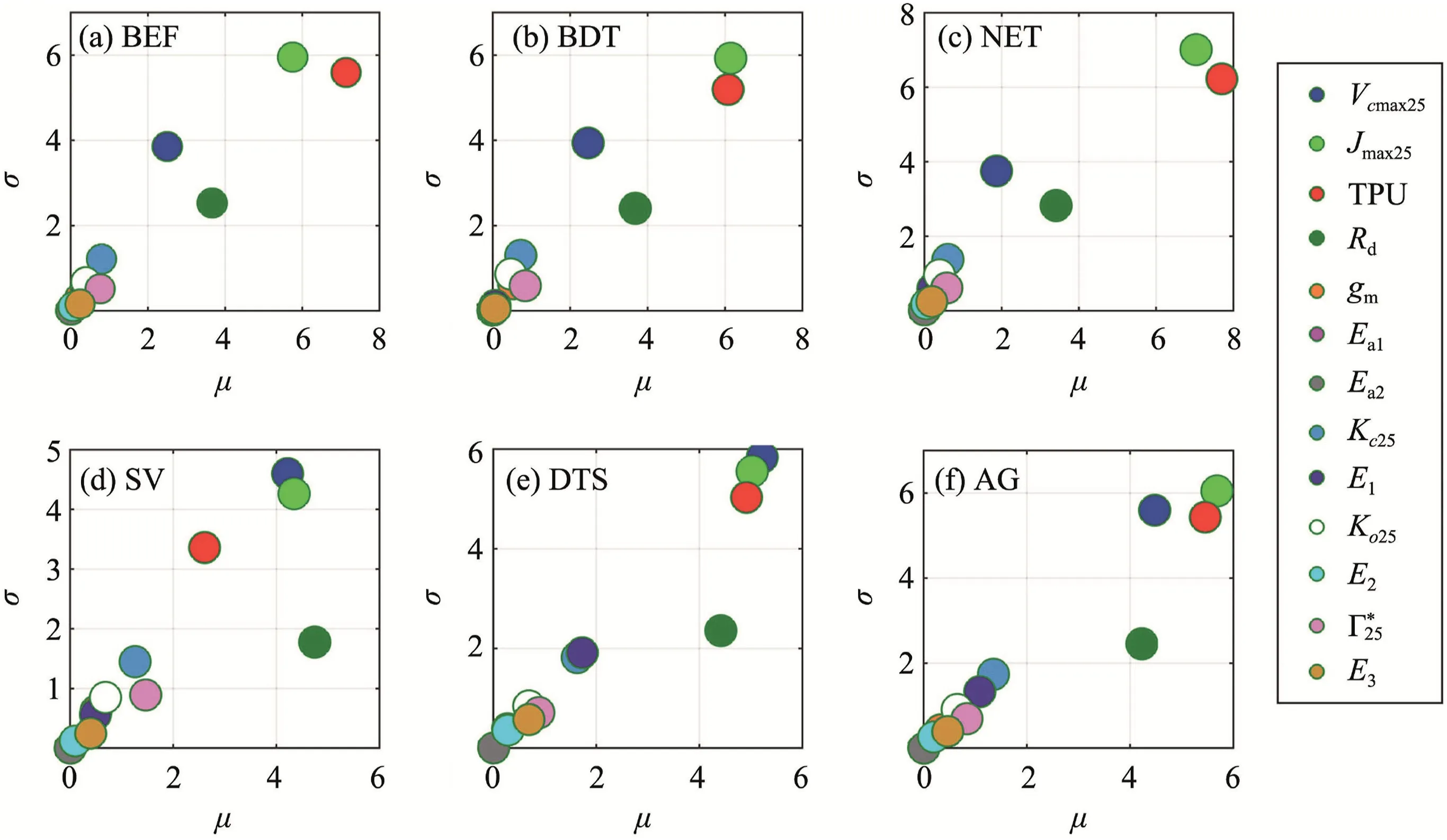
Fig.3.Morris scatter diagram of 13 parameters in six vegetation types (a) BET, (b) BDT, (c) NET, (d) SV, (e) DTS, and (f) AG, respectively.

Here, the accumulating contribution rate was used to test the effectiveness of SA result in the Morris method (Fig.4).Results show that effectiveness of the two most sensitive parameters could reach about 50%,and the four most sensitive parameters could reach more than 90%for vegetation belonging to SV, DTS and AG (Figs.4d, 4e, 4f).For BET,BDT and NET,the two most sensitive parameters provided a contribution rate of more than 90%(Figs.4a,4b, 4c).

Fig.4.The accumulating contribution rate of 13 parameters to model output in six vegetation types.(a) BET, (b) BDT, (c) NET, (d) SV, (e) DTS, and (f) AG,respectively.

3.3.Sensitivity analysis based on different objective functions

In order to verify if the objective functions would affect sensitive parameters identification using the two SA methods,results based on the Sobol’method and the Morris method with different statistical goodnessof-fit metrics (i.e., RMSE, NSE, and STDEV) were compared (Figs.5 and 6).In Fig.5,each column from left to right represented sensitivity indices with objective functions RMSE,NSE,and STDEV,respectively.Obviously,model output based on the Sobol’ method with metric RMSE was consistent with model output with metric NSE (Fig.5).Only two parameters(i.e.,Jmax25and TPU)were sensitive,whose total-order indices were larger than 10%for BET,BDT,and NET(Figs.5a,5d,5g for metric RMSE; Figs.5b, 5e, 5h for metric NSE).Four parameters (i.e., Vcmax25,Jmax25, TPU, and Rd) were sensitive, whose total-order indices were larger than 10%for SV,DTS,and AG(Figs.5j,5m,5p for metric RMSE;Figs.5k,5n,5q for metric NSE).Similarly,the Morris method confirmed that objective functions RMSE and NSE would produce consistent SA results (Fig.6).

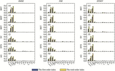
Fig.5.First and total-order indices for 13 parameters with different objective functions(i.e.,first,second,and third columns represent sensitivity indices with RMSE,NSE,and STDEV,respectively);x-axis represents parameters(detail information is summarized in Table 1);(a–c)BET,(d–f)BDT,(g–i)NET,(j–l)SV,(m–o)DTS,and(p–r) AG, respectively.

Fig.6.Morris scatter diagram of 13 parameters with different objective functions (i.e., first, second, and third column represent sensitivity indices with RMSE,NSE,and STDEV, respectively); (a–c) BET, (d–f) BDT, (g–i) NET, (j–l) SV, (m–o) DTS, and (p–r) AG, respectively.

Differently, model output with objective function STDEV was different from that with objective function RMSE and NSE(Figs.5c,5f,5i,5l, 5o, 5r).Firstly, interaction effect of each parameter to others was more apparent,i.e.,difference between total-and first-order indices was much larger than that when objective function was RMSE or NSE.Secondly, when objective function was RMSE or NSE, SA results of vegetation belonging to BET, BDT, NET were different from SA results of vegetation belonging to SV, DTS, AG.In contrast, when the objective function was STDEV,SA results of vegetation among all six PFTs show no obvious difference.Furthermore,results based on the Morris method also show a significant difference between model output with objective function STDEV and model output with objective function with RMSE or NSE(Figs.6c, 6f,6i,6l, 6o,6r).

4.Discussions

4.1.Model mechanism of the FvCB model

The primary objective of this paper was to identify sensitive parameters of all parameters in the FvCB model.Not surprising,two parameters(the maximum electron transport rate at 25°C,Jmax25,and the maximum rate of Rubisco activity at 25°C,Vcmax25)were the most sensitive across all plant functional types.Here,we found that there were four sensitive parameters(total-order index>10%of parameters Vcmax25,Jmax25,TPU,and Rd) for vegetation belonging to SV, DTS, and AG, while there were only two sensitive parameters (total-order index >10% of parameters Jmax25and TPU) of all 13 parameters for vegetation belonging to BET,BDT,and NET.Photosynthesis process was divided into three stages,i.e.,the light reaction stage,the dark reaction stage and the C-concentrating stage (Long and Bernacchi, 2003; Atkin et al., 2016).Thus, photosynthesis was limited to three potential factors, i.e., Rubisco-limited, RuBP regeneration-limited and triose phosphate use-limited factor in the FvCB model(Farquhar et al.,1980;Harley et al.,1986;Rogers et al.,2017).In light reaction stage, radiant energy is absorbed by chlorophyll, then accessory pigments clinging to the chloroplast lamella membranes help to generate a kind of high-energy compounds (i.e., adenosine triphosphate,ATP)(Shi et al.,2020).In the second stage,as the receptor of CO2,ribulose bisphosphate (RuBP) is fixed by ribulose 1,5-bisphosphate carboxylase/oxygenase(Rubisco).It was confirmed that the maximum rate of Rubisco activity(Vcmax) was mainly controlled by activity of Rubisco(Lloyd et al.,1992;Medlyn and Dreyer,2002;Wullschleger et al.,2014).Based on the Arrhenius theory,Vcmaxcan be expressed by an exponential equation with parameter Vcmax25and a kind of activation energy parameter Ea1.Parameter Vcmax25controlled the discretion and Ea1controlled the exponential rising rate.Thus, Vcmax25was a very key parameter, and the variation of Vcmax25would have a significant influence on model output.

In the Calvin cycle,another important process in dark reactions stage is triose phosphate regeneration (von Caemmerer and Farquhar, 1981;Bernacchi et al., 2001).After a series of chemical conversion, ribulose bisphosphate (RuBP) and triose phosphate (TP) are generated, during which RuBP regeneration is limited either by electron transport rate or triose phosphate use (TPU).Thus, the light-saturated rate of electron transport (Jmax) and the rate of triose phosphate use (TPU) became key parameters.Mitochondrial respiration (Rd) was another critical process in photosynthesis which included a series of substrate oxidation(Sharkey et al.,2007;Fisher et al.,2015).A variety of enzymes related to substrate oxidation producing mitochondrial respiration is highly sensitive to the environment.

4.2.Comparison of the Sobol’ method and the Morris method

Parameter SA is an effective technology to asses'responses of model output to the variation of parameters,which is beneficial to concentrate efforts on calibrating sensitive parameters(Bonan et al.,2011;Orr et al.,2016).Typically, parameter SA methods can be classified into two categories:qualitative SA and quantitative SA methods.The former aims for sensitivity ranking, rather than quantification of variance contribution,which are efficient and effective(Nossent et al.,2011).The latter aims to quantify uncertainty of the output caused by variations of input factors(Han and Zheng,2016).Here,we compared a qualitative(i.e.,the Morris method) and a quantitative (i.e., the Sobol’ method) SA method to identify sensitive parameters in the FvCB model.The sensitivity analysis exhibited that the net CO2assimilation rate was sensitive to 4 of the 13 parameters (i.e., Vcmax25, Jmax25, TPU, and Rd).Also, comparable results using the NSE and STDEV goodness-of-fits suggested that our approach is reliable (Figs.5 and 6).

The Sobol’ method is a typically variance based on the Monte Carlo method which can explain how individual parameter and their interaction effect performance of the impact model.This method has the advantage of treating grouped input factors such as the interaction effect.Meanwhile,intervention of the Latin hypercube sampling method has a large improvement in sampling efficiency(Hall et al.,2005;Zhang et al.,2013).In recent years,this method has been broadly used in many fields.Compared with the Sobol’method,the Morris method is an economic SA method.The modified mean(μ)assesses the sensitivity strength between the ithinput variable and the output.Meanwhile,σ is used to determine possible interactions with other variables (Morris, 1991; Campolongo et al.,2007).In this paper,it has been confirmed that the Morris method is efficient in identifying sensitive parameters.Also, insensitive parameters can be fixed at empirical values, reducing the workload of further optimization(Patrick et al.,2009;Orr et al.,2016;Franks et al., 2018).

4.3.Results affected by different objective functions

In order to identify whether the objective function had any impact on the result of model parameter sensitivity, RMSE, NSE, and STDEV were used as statistical goodness-of-fit metrics.In both the Morris method and the Sobol’ method, the direct model output (f) is replaced by a model goodness-of-fit metric.Generally, objective function expresses the proximity of model simulation results compared with observations in a time series.In many hydrological models, metric RMSE is commonly used as objective function, and a smaller value of objective function meant a better model fit(Tarin et al.,2020).NSE is another broadly used objective function in model parameter optimization.The closer of NSE value, the better model fit.When the NSE value is near to 0,the goodness of fit of simulation to observation is close to the average value of observation sequence(Tang et al.,2007;Medlyn et al.,2017).Metric STDEV expresses a deviation degree between sequence simulated by model and observation sequence in the corresponding period.

In this paper, both the Morris method and the Sobol’ method show significant difference between model output with objective function STDEV and model output with objective function with RMSE or NSE(Figs.5 and 6).The reason for causing a difference between sensitivity results when objective function is STDEV and objective function is RMSE or NSE is that metric Standard Deviation only considers simulation value and neglects observation value, leading to discrepant results.Thus, we recommend statistical goodness-of-fit metrics RMSE and/or NSE as the objective function when conducting parameter SA based in the Sobol’method and the Morris method.

5.Conclusions

This paper tested two global parameter sensitivity analysis approaches,i.e., the Sobol's method and the Morris method,in conducting parameter SA of the FvCB model.A quantitative analysis including individual and interactions effect based on the Sobol’method,and a qualitative analysis of the Morris method based on statistical goodness-of-fit metrics RMSE,NSE and STDEV were compared.It was confirmed that only a small part of model parameters in the FvCB model were sensitive, which show variations among PFTs.The two SA methods used in this paper successful identified key parameters,and provide reliable and consistent results.The Morris method screened out sensitive parameters qualitatively based on a relatively small sample size,while the Sobol’method quantified sensitivity indices and sensitivity rankings.Parameter SA with statistical goodness-offit metrics RMSE and NSE exhibited similar performance, while the SA result with STDEV was significantly different.Thus, we would prefer to statistical goodness-of-fit metrics RMSE and NSE as objective functions in SA of the FvCB model.Our findings provide a new insight into model parameter optimization in the photosynthetic part of LSMs.

Acknowledgements

This study was supported by the CAS"Light of West China"Program(No.[2020]82),Key technology projects of Inner Mongolia Autonomous Region(Grant No.2020GG0306),Science and Technology Plan Projects of Alxa League(Grant No.AMY2020-18)and Natural Science Foundation of Gansu Province(No.21JR7RA038).

Code of the Sobol' method

clc

clear

Nss=10000;%Sample numbers

load data

y_obs=data(:,1);

ci =data(:,2);

T = data(:,3);

%Prior parameter interval for

%Vcmax25,Jmax25,TPU,gm,Ea1,Ea2,Kc25,E1,Ko25,E2,f125,E3,

Rd25,E4

interval=[];

dem=size(interval,1);%dimension of parameter vector

%Generate matrices A and B using the LHS technique

[Am,Bm]=LHSsample(Nss,dem,interval);

%calculate the sensitivity index

sa1=0;

sb1=0;

ss1=zeros(1,dem);

st1=zeros(1,dem);

AB=zeros(1,dem);

for j=1:Nss

y_s1=Farquhar(Am(j,1),Am(j,2),Am(j,3),Am(j,4),Am(j,5),Am(j,6),

Am(j,7),Am(j,8),Am(j,9),Am(j,10),Am(j,11),Am(j,12),Am(j,13),ci,T);

AnA=Bias(y_obs,y_s1,length(T));

sa1=sa1+AnA;

sb1=sb1+AnA^2;

bfo(j,1)=sa1/j;

VY(j,1)=sb1/j-bfo(j,1)^2;

y_s2=Farquhar(Bm(j,1),Bm(j,2),Bm(j,3),Bm(j,4),Bm(j,5),Bm(j,6),

Bm(j,7),Bm(j,8),Bm(j,9),Bm(j,10),Bm(j,11),Bm(j,12),Bm(j,13),ci,T);

AnB=Bias(y_obs,y_s2,length(T));

for i=1:dem

AB=Am(j,:);

AB(i)=Bm(j,i);

y_s3=Farquhar(AB(1),AB(2),AB(3),AB(4),AB(5),AB(6),AB(7),AB(8),

AB(9),AB(10),AB(11),AB(12),AB(13),ci,T);

AnAB=Bias(y_obs,y_s3,length(T));

ss1(i)=AnB＊(AnAB-AnA)+ss1(i);

Si(j,i)=ss1(i)/(j＊VY(j,1));

st1(i)=st1(i)+(AnA-AnAB)^2;

ST(j,i)=st1(i)/(2＊j＊VY(j,1));

end

end

%%figure plot

%Si plot

Sii=Si(5:end,:);

figure1= figure(1);

%Create axes

axes1 =axes(‘Parent’,figure1,‘YGrid’,‘on’,‘XGrid’,‘on’);

box(axes1,‘on’);

hold(axes1,‘all’);

plot1=plot(Sii,‘DisplayName’,‘Sii’,‘YDataSource’,‘Sii’);

%set(plot(1),‘DisplayName’,‘Sii(:,1)’);

%set(plot(2),‘DisplayName’,‘Sii(:,2)’);

%set(plot(3),‘DisplayName’,‘Sii(:,3)’);

%set(plot(4),‘DisplayName’,‘Sii(:,4)’);

% set(plot(5),‘DisplayName’,‘Sii(:,5)’);

legend(axes1,‘show’);

%St plot

STT=ST(5:end,:);

figure2= figure(2);

%Create axes

axes2 =axes(‘Parent’,figure2,‘YGrid’,‘on’,‘XGrid’,‘on’);

box(axes2,‘on’);

hold(axes2,‘all’);

plot2=plot(STT,‘DisplayName’,‘STT’,‘YDataSource’,‘STT’);

%set(plot2(1),‘DisplayName’,‘STT(:,1)’);

%set(plot2(2),‘DisplayName’,‘STT(:,2)’);

%set(plot2(3),‘DisplayName’,‘STT(:,3)’);

% set(plot2(4),‘DisplayName’,‘STT(:,4)’);

%set(plot2(5),‘DisplayName’,‘STT(:,5)’);

legend(axes2,‘show’);

Code of the Morris method

%%para_in

clc

clear all

load data

y_obs=data(:,1);

ci =data(:,2);

T =data(:,3);

k=input(‘Enter the K(NO.of factors):’);

p=input(‘Enter the P(NO.of levels):’);

r=input(‘Enter the R(NO.of samples):’);

%%22^I^Eý£¡£¡£¡

%

interval=[];

aa=interval(:,1)’;

bb=interval(:,2)’;

%%

h=waitbar(0,‘Ǩe′E^Oµ‵E£¬~Oý^OÚ×¼±¸¼Æ¨E~a...’);

%tic

for i=1:r

[Bstar delta a d]=zk1(p,k,r,aa,bb);

%Call model

for j=1:d

[y_s1]=Farquhar(ci,T,Bstar(j,:));

[y_s2]=Farquhar(ci,T,Bstar(j+1,:));

p1=NSE(y_obs,y_s1);

p2=NSE(y_obs,y_s2);

eei(i,a(j))=abs(p1-p2)/delta;

end

waitbar(i/r,h,‘Ǩeµ‵E′ý...‵A2‵A2‵A2~~~~’);

end

waitbar(1,h,‘‵O~N′I^e3′E£¡£¡£¡’);

pause(1);

delete(h);

%t=toc

%disp(t)

%%Get the mean and standard deviation of the elementary effects.

mycolor=[];

for i=1:k

mu(i)=mean(eei(:,i));

sigma(i)=std(eei(:,i));

end

for i=1:length(mu)

scatter(mu(i),sigma(i),104,‘MarkerFaceColor’,mycolor(i,:),...

‘MarkerEdgeColor’,[0 0.5 0])

hold on

grid on

end

mu=mu’;

sigma=sigma’;