Modelling and applications of dissolution of rocks in geoengineering

Farid LAOUAFA, Jianwei GUO, Michel QUINTARD

Research Article

Modelling and applications of dissolution of rocks in geoengineering

Farid LAOUAFA1*, Jianwei GUO2*, Michel QUINTARD3,4

1National Institute for Industrial Environment and Risks (INERIS), Verneuil en Halatte, 60550, France2School of Mechanics and Aerospace Engineering, Southwest Jiaotong University, Chengdu 610031, China3Université de Toulouse, INPT, UPS, IMFT (Institut de Mécanique des Fluides de Toulouse), Allée Camille Soula, Toulouse, F-31400, France4CNRS, IMFT, Toulouse, F-31400, France

The subsoil contains many evaporites such as limestone, gypsum, and salt. Such rocks are very sensitive to water. The deposit of evaporites raises questions because of their dissolution with time and the mechanical-geotechnical impact on the neighboring zone. Depending on the configuration of the site and the location of the rocks, the dissolution can lead to surface subsidence and, for instance, the formation of sinkholes and landslides. In this study, we present an approach that describes the dissolution process and its coupling with geotechnical engineering. In the first part we set the physico-mathematical framework, the hypothesis, and the limitations in which the dissolution process is stated. The physical interface between the fluid and the rock (porous) is represented by a diffuse interface of finite thickness. We briefly describe, in the framework of porous media, the steps needed to upscale the microscopic-scale (pore-scale) model to the macroscopic scale (Darcy scale). Although the constructed method has a large range of application, we will restrict it to saline and gypsum rocks. The second part is mainly devoted to the geotechnical consequences of the dissolution of gypsum material. We then analyze the effect of dissolution in the vicinity of a soil dam or slope and the partial dissolution of a gypsum pillar by a thin layer of water. These theoretical examples show the relevance and the potential of the approach in the general framework of geoengineering problems.

Dissolution; Modelling; Scaling; Evaporite; Deformation; Plasticity

1 Introduction

Natural or human induced dissolution of soluble rocks in contact with water affects many soils and subsoils. These perturbations result in a redistribution of the effective or total stress field and thus the deformation of the soil and subsoil. The mechanical response of the soil and its impact on the surface depend on the location and the geometric features of the cavities resulting from dissolution. This damage is mainly related to the "change of phase", from solid to liquid, of part of the domain.

With this change, the stress field can reach critical states with plasticity or failure in part of the domain in question. Examples of potential effects include subsidence, sinkholes, and impacts on geo-structures (James and Lupton, 1978; Bellet al., 2000; Swift and Reddish, 2002; Waltham et al., 2005; Castellanza et al., 2008; Gerolymatou and Nova, 2008). Particular attention must be paid to the understanding and control of this phenomenon, which is very important in geoengineering contexts.

An intrinsic difficulty in the dissolution of underground rocks is the time dependency of the geotechnical problem, but there is a lack of in-situ data concerning its evolution in space and time. Rock dissolution occurs as long as the fluid flow in the subsurface is undersaturated. In this study we will concentrate mainly on the dissolution of gypsum rocks (CaSO4·2H2O), even though the numerical approach implemented to describe dissolution has a broader scope. Therefore, we also include reference to some problems involving salt (NaCl). A substantial contrast between a problem involving salt and one involving gypsum is their solubilities and the corresponding physical instabilities. We note that the solubility, defined as the maximum amount of a chemical species that dissolves in a specified amount of solvent (water) at a prescribed temperature, of evaporites can range over several orders of magnitude. For example, the solubilities of salt, gypsum, and limestone are 360, 2.50, and 0.013 g/L, respectively (Freeze and Cherry, 1979).

Answering the questions posed by the dissolution process is a difficult and non-trivial exercise. Indeed, the problem exhibits several multi-scale and multi-physical features, couplings, and non-linearities. One difficulty is related to the precision required in the description and quantification of the recession rate of the solid-liquid interface at the macroscopic scale. To circumvent this scientific drawback, a specific mathematical statement of the physico-chemical and transport equations at the microscopic or pore scale is established. Another difficulty is to tackle dissolution phenomena at in-situ or geo-structure scales. Such problems are linked to the strong physical coupling with other processes, such as the mechanical behavior of rocks. In contrast to the phenomenological or "averaged" approaches to the dissolution process (Jeschke et al.,2001; Jeschke and Dreybrodt, 2002), our approach begins at the microscopic scale.

In this study we briefly present the approach proposed to model and solve the dissolution problem. The method is built on a strong theoretical basis but is also supported by numerical modelling. The mathematical formalization of the problem of the dissolution surface and its kinetics are initially built at the pore scale. A possible candidate numerical approach to describe dissolution is a method that explicitly follows the fluid-solid interface. The arbitrary Lagrangian-Eulerian (ALE) method proposed by Donea et al. (1982) is well suited to that. An alternative approach no longer views the interface as a sharp and discontinuous boundary between solid and liquid but considers the interface to have a finite thickness and well-defined properties (notably continuity); in other terms, it is a diffuse interface (Collins and Levine, 1985; Anderson and McFadden, 1998). We limit our development to two-phase porous media and we assume fluid-saturated porous rocks.

We present the physical and mathematical basis of the pore-scale dissolution model and the upscaled diffuse interface model (DIM) using a volume-averaging theory. The part of this study which is dedicated to the geomechanical consequences considers only gypsum rocks. Whatever the hydrogeological configuration, the dissolution of gypsum (lenses, pillars, etc.) in the ground raises questions in terms of geomechanical consequences: subsidence, sinkholes, stability of pillars or cavities, etc. (Toulemont, 1981, 1987; Cooper, 1988; Bell et al., 2000; Gysel, 2002). The aim of the last section of this paper is to show, by several 2D and 3D theoretical examples, the robustness and the potential of the proposed numerical dissolution approach.

The geotechnical problems to be addressed are elastoplastic ones. The elastoplastic constitutive models used to describe the behavior of soil and gypsum are relatively simple. The aim is not to develop a precise study of a real case but to provide an illustration of the ability of the proposed approach. This is valid regardless of the complexity of the constitutive model used. We will illustrate these issues in the case of plasticity within a soil mass in the vicinity of a dike and in the case of partial dissolution of an elastoplastic pillar. In all the studied configurations, the soluble gypsum is located inside porous domains.

We can see from the numerical modelling that the proposed approach has a predictive aspect. Indeed, the mechanical and dissolution coupling allows us to model the time evolution of all the fields (stresses, strains, displacements, etc.) and to determine the critical time beyond which severe risks can appear. In this study only the DIM method will be used in the different examples.

2 Mathematical formulation of the dissolution

This section is devoted to a brief review of the underlying principles of the method used for modeling the dissolution. The reader can find more detailed information on the scientific background in (Luo HS et al., 2012, 2015; Luo H et al., 2014; Guo et al., 2015, 2016). At the pore scale, the dissolution problem can be posed using the classical initial and boundary-value problems. To achieve the expression of the "macro" DIM model, we start with these "small-scale" equations to generate Darcy-scale equations, the corresponding Darcy-scale quantities, and effective coefficients, using volume-averaging theory (Whitaker, 1999). After introducing the original model (micro-scale) for the dissolution problem, we present an upscaling method leading to the "Darcy-scale" equations.We provide a quick review of the main ideas and principles on the upscaling of the pore-scale equations to the macroscopic scale. The Darcy-scale model derived from this upscaling is the one that is used for large-scale dissolution modeling. The passage of the description of the phenomena from the microscopic to the real "geotechnical" scale is depicted in Fig. 1.

Before going further, note that we restrict our discussion to porous media composed of two phases, a solid skeleton (solid phase) and a liquid phase. The porous medium is fully saturated with liquid. More general approaches can be found in (Luo HS et al., 2012; Luo H et al., 2014). To distinguish the phases, we will use the subscript "s" to indicate the solid phase and the subscript "l" to indicate the liquid phase.

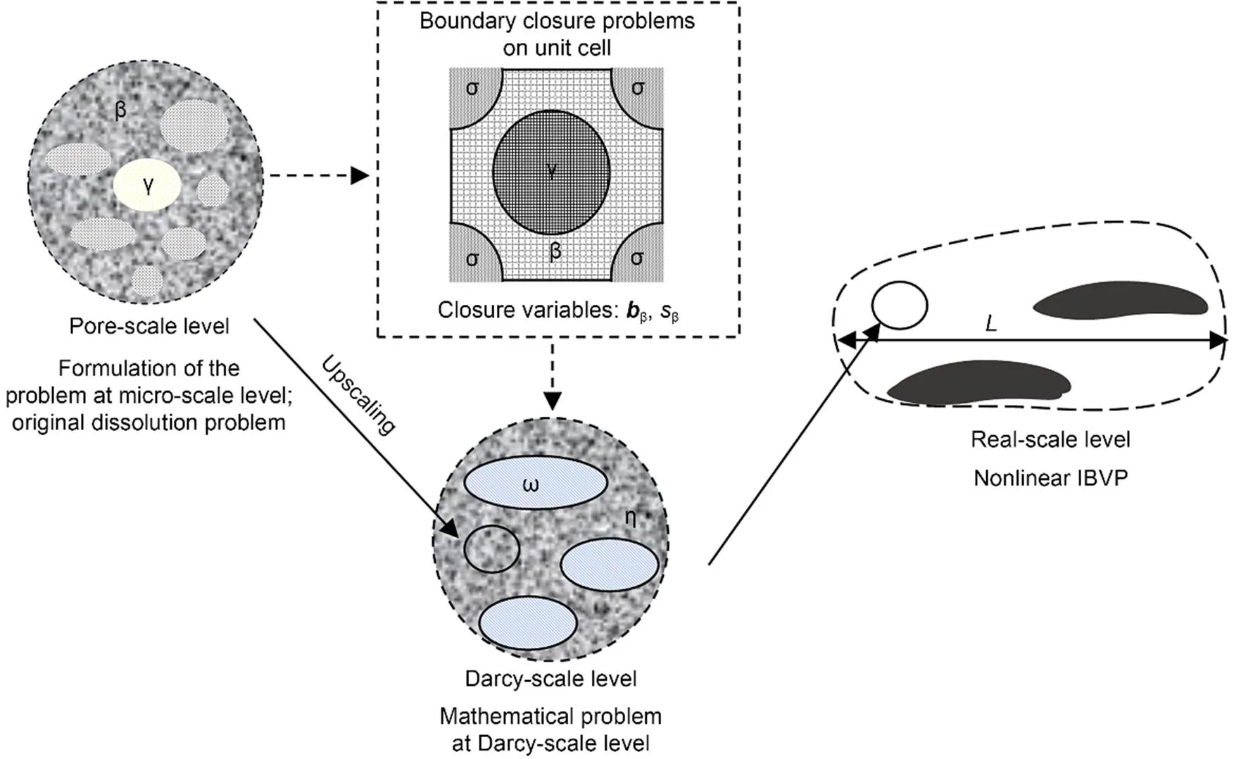
Fig. 1 Sketch of the passage from microscopic to real in-situ scales, closure variables, and 2D unit cell. The general notations β, γ, ω, σ, and η indicate different phases (fluid, soluble phase, heterogeneities, non-soluble phase, …). bβ and sβ are solutions of the boundary value closure problems, and L is the large-scale length. IBVP refers to the initial boundary value problems

2.1 Pore-scale model

Let us consider a binary liquid phase l containing chemical species A and B, and a solid phase s containing only chemical species A, as depicted in Fig. 3 (right).

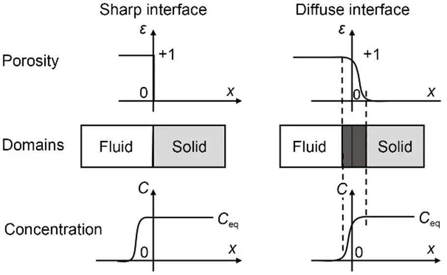
Fig. 2 ‍Porosity ε and concentration C space-evolution when crossing a sharp and a diffuse interface. Fig. 2 is reprinted from (Laouafa et al., 2021), Copyright 2021, with permission from Springer Nature

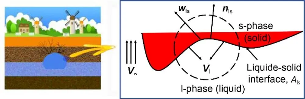
Fig. 3 Sketch of in-situ cavity and focus near a rock-solid/fluid interface. nls is the normal outward vector, wls is the interface or recession velocity, and V∞ is the velocity far from the interface

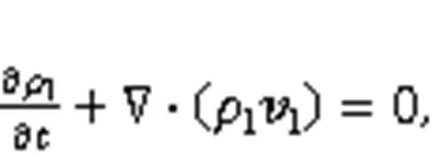
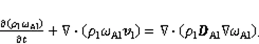
wherel,s,l,s,Al, andAlare the density of l-phase, density of s-phase, the l-phase velocity, the s-phase velocity, the mass fraction of species Ain the liquid, and the diffusion tensor, respectively.

In the following analysis, the s-phase is supposed immobile (s=0). The momentum balance for the fluid follows the Navier-Stokes equations:

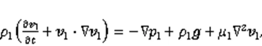
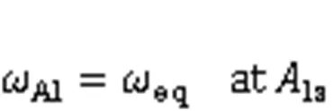
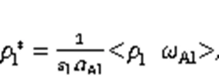
wherelrepresents the water pressure in the l-phase,lis the liquid dynamic viscosity, andis the gravity vector. Under some assumptions (Luo et al., 2012), we have the classical equilibrium conditioneqat the fluid/solid interfacels, i.e.,

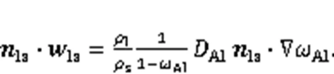
The boundary conditions for the mass balance at the solid-liquid interface with normal outward vectorlscan be written as follows (Fig. 3) (atls):

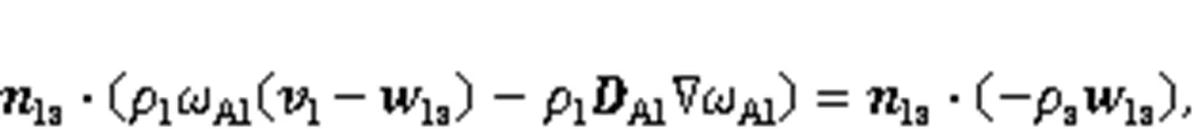
wherelsis the interface or recession velocity. This equation may be used for instance to compute explicitly the interface velocity in the ALE method and can be expressed as follows:

2.2 Upscaled macro-scale non-equilibrium model

A DIM model can be written in an appropriate way in the framework of porous medium theory. In this subsection, we describe the macroscopic Darcy-scale equations obtained by upscaling the above set of pore-scale equations, using the volume averaging theory (Quintard and Whitaker, 1994a, 1994b, 1999). The reader will find the details of this change of scale in (Guo et al., 2016). The representative elementary volumes (Bachmat and Bear, 1987) are illustrated in Fig. 4. We define the intrinsic average of the mass fractionAland the superficial average of the velocitylas

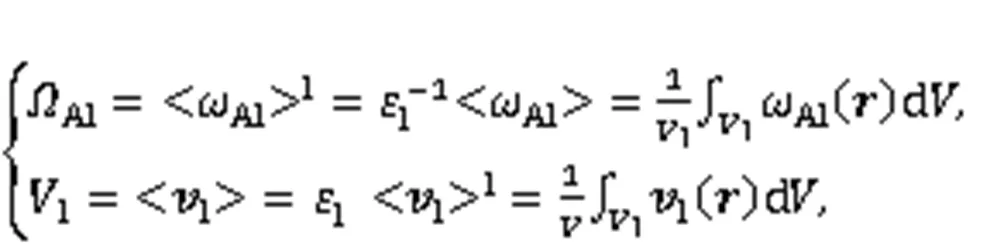
Fig. 4 Averaging volume at pore-scale level. rβ is the position vector locating points in the β-phase, and yβ is the position vector locating points in the β-phase relative to the centroid

whereis the averaging volume andis the position vector locating points in the β-phase.

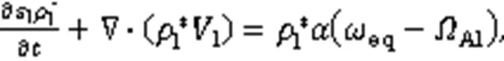
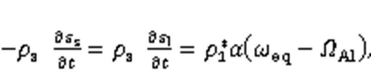
After transformation, the averaged form of the balance equation of species A can be expressed as

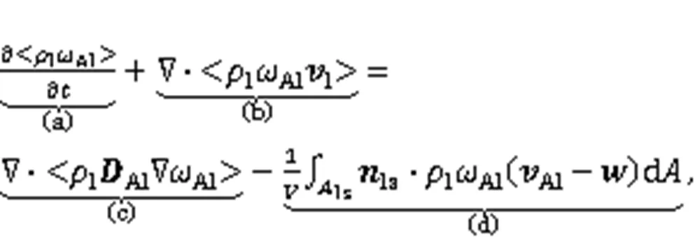
where (a), (b), (c), and (d) represent the accumulation, the convection, the diffusion, and the phase exchange terms, respectively. With several assumptions and some mathematical manipulations of the various equations, we derive the following equations for the DIM model (Luo et al., 2012):

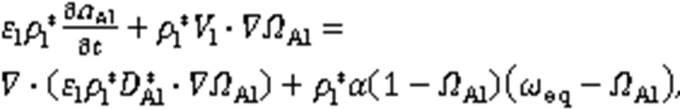
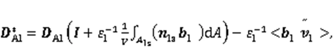
The values of the macroscopic effective coefficients (values at the Darcy-scale) are obtained thanks to the solution of the "closure problems" over a unit cell, whose shape and topology are specific to the porous medium being considered, as pictured in Fig. 5.

Their expressions according to Luo et al. (2012) are:

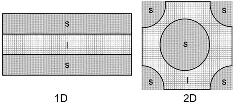
Fig. 5 ‍Pictures of unit cells defining the domain of the closure problems

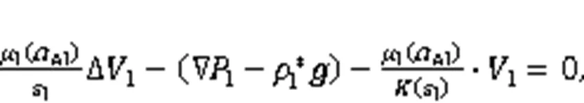
At this scale, the fluid velocity can be described either by the classical Darcy model or the Darcy-Brinkman version (Brinkman, 1949):

In the following section, we illustrate the use of the methodology in the analyses of some dissolution examples.

2.3 Modelling of direct leaching process in a salt mass

This section discusses the application of the proposed approach described in the above section. The first application consists in the modeling of a direct leaching test performed in a salt mass. We compare the results of the modeling to the experimental measures. The goal is to illustrate the capacity of the approach to face problems with geometrical singularity and important density impacts resulting from high salt solubility.

The principles of the experimental in-situ test are as follows. Two concentric tubes are driven into the ground to a depth of 280 m (Fig. 7a). Through the central tube, water is injected continuously for several days. The injection by the central tube is known as the direct leaching method. The injection history is given in terms of velocity in Fig. 7c and is 3 m3/h for 4 d and 1.5 m3/h for 8 d. A sonar test of the dissolution void was carried out and it was deduced that the final form of the cavity obtained was quasi-cylindrical as illustrated in Fig. 7b.

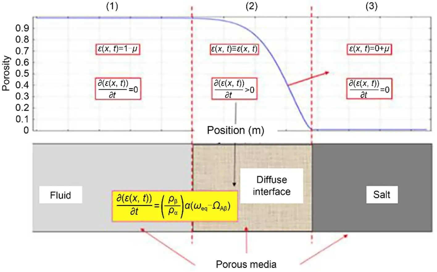
Fig. 6 Porosity evolution and rate condition in the whole porous media including the diffuse interface. Reprinted from (Laouafa et al., 2021), Copyright 2021, with permission from Springer Nature

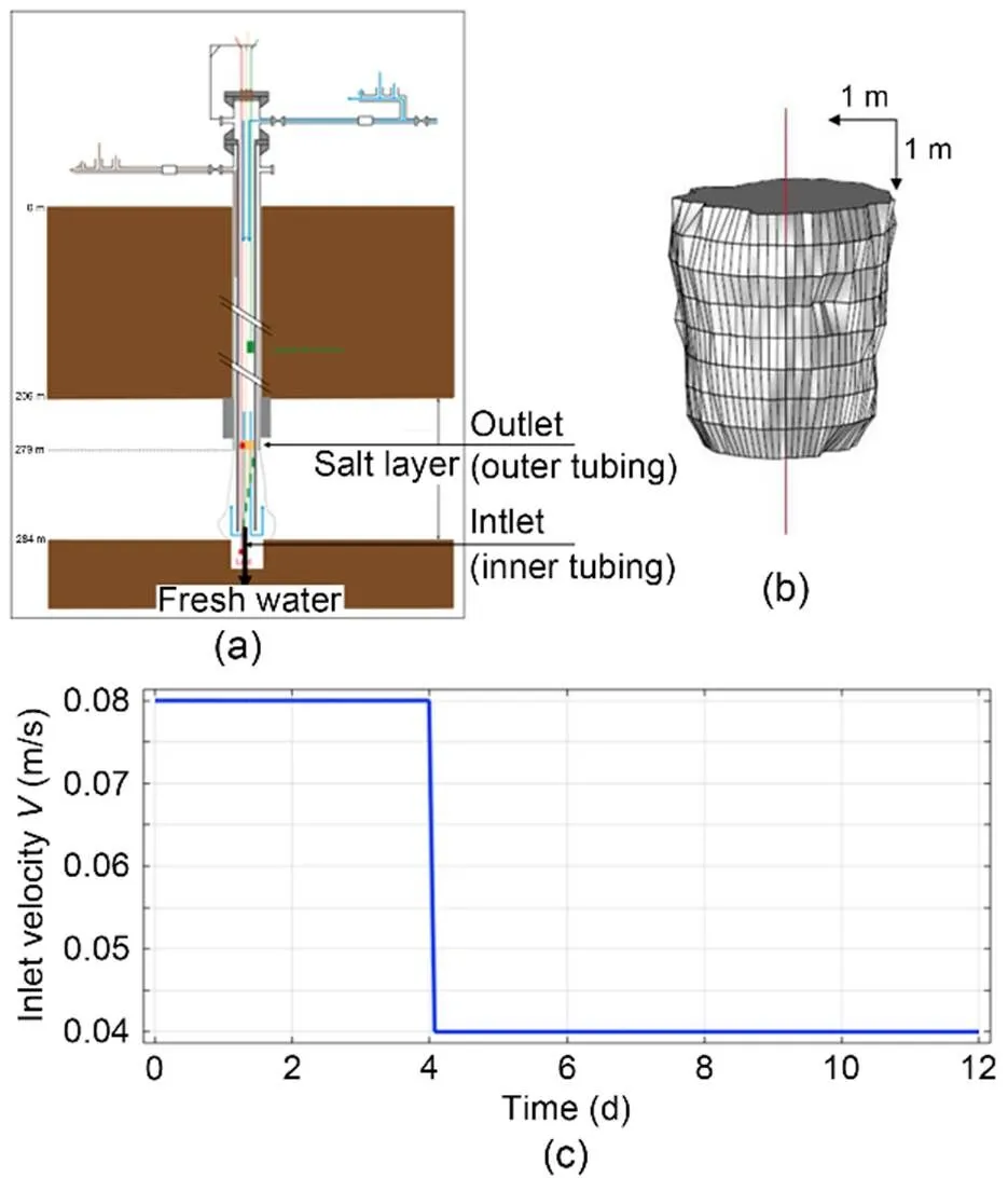
Fig. 7 Configuration of the experimental leaching test (a), resulting dissolution after 12 d of freshwater injection (b), and inlet velocity history (c) (Charmoille and Daupley, 2012)

In the numerical modelling of this direct leaching process, we first suppose that the problem is axisymmetric. Proper initial and boundary conditions describing this problem are applied in the numerical model, which was solved using the finite element method. The liquid (brine) densityl(kg/m3) has the following expression:

whereAl(,) is the mass fraction of species Aat timeand point. The mass fraction at equilibriumeqis equal to 0.27. The salt densitysis equal to 2165 kg/m3. The liquid dynamic viscositylis supposed constant and equal to 1.0×10-3Pa·s and the diffusivity is equal to 1.3×10-9m2/s. The permeability of the salt rock is equal to 1.0×10-20m2. The numerical results of this experimental test are shown hereafter. Fig. 8 shows, at different times, the value of the porosity inside the domain in the axisymmetric plane. We observe on this figure the development of a near-cylindrical cavity, a shape that is maintained over time. The gradient of color between the "fluid" part (red) and the "solid part" (blue) indicates the existence of a diffuse interface of a finite width.

The computed dissolved volumes are around 12 m3after 4 d and 38 m3after 12 d. The experimental evaluations of the cavity volume deduced from the outlet fluid composition analysis are around 11 m3and 40 m3, respectively. This demonstrates the accuracy of the numerical model.

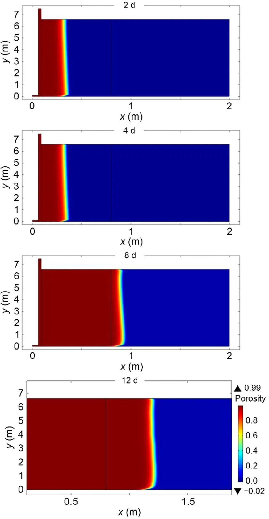
Fig. 8 Iso-value of the porosity after 2, 4, 8, and 12 d (void, fluid filled cavity, is red). References to color refer to the online version of this figure

The flowlines (Fig. 9) show at different times or cavity volumes, the natural convection effect linked to concentration (mass fraction) gradients due to the strong solubility of salt. Such natural convection effects are also reported in (Wang et al., 2021).

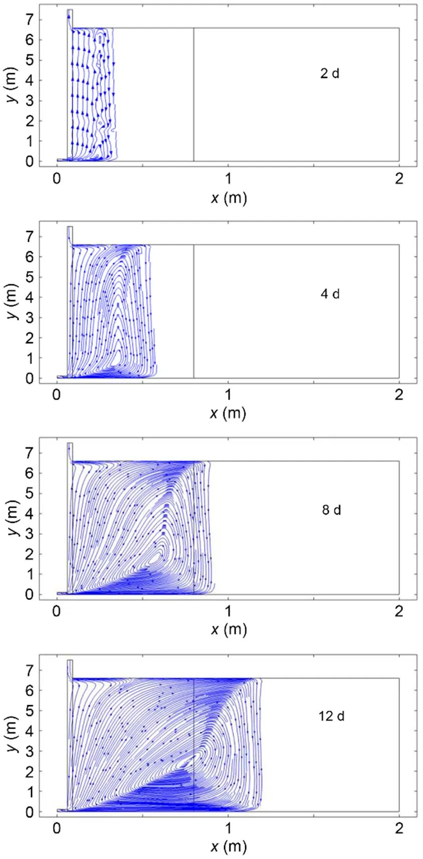
Fig. 9 Streamlines and fluid vector fields after 2, 4, 8, and 12 d

In Fig. 10, we have represented the position of the liquid/salt interface at six instants. In this point tracking, we have considered the interface situated at mid-height (segment AA). It is noteworthy that the interface is not sharp but has a finite thickness.

With the same boundary conditions as above, we consider now, instead of salt, a gypsum domain and its associated parameters (Guo et al., 2016). In these computations, the liquid density is kept constant (very small solubility) and equal to 1000 kg/m3. Fig. 11 shows the cavity at different times (1, 5, 10, and 30 a). We observe the very slow dissolution rate (small cavity after a long time) for gypsum material and the different cavity shapes compared to those obtained with salt.

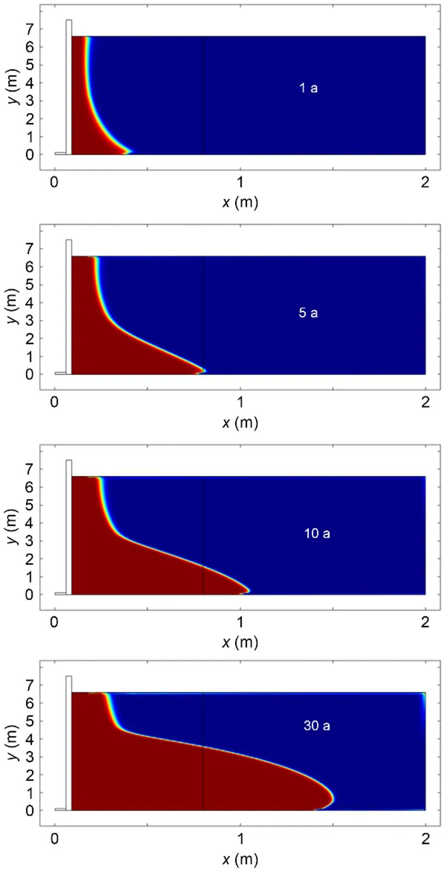
Fig. 11 Shapes of the cavity in gypsum after 1, 5, 10, and 30 a (void is red). References to color refer to the online version of this figure

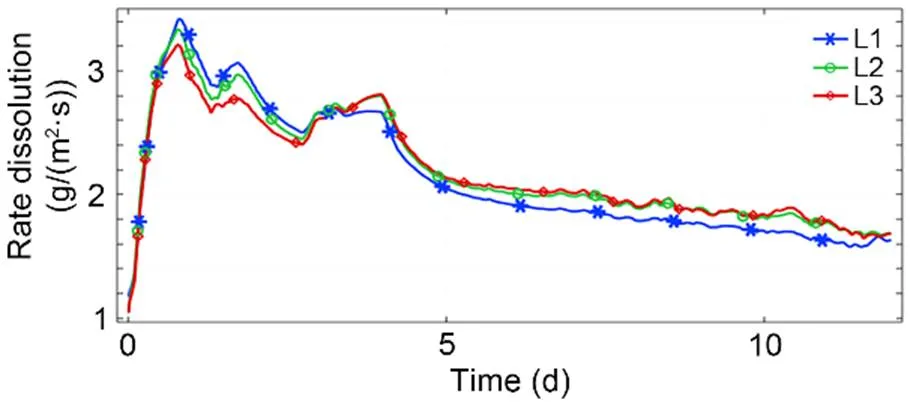
Fig. 12 Time evolution of the recession rate along three lines located in the salt layer (bottom-L1, middle-L2, top-L3) for the case of direct leaching process in salt mass (Fig. 7)

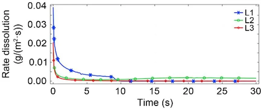
Fig. 13 Time evolution of the recession rate along three lines located in the gypsum layer (bottom-L1, middle-L2, top-L3) for the case of direct leaching process in salt mass (Fig. 7)

We can observe that the recession rate is far from being constant in time either for salt or for gypsum. So, it does not make sense to use a unique and constant value for the dissolution rate, as is often done in engineering practice, since it evolves according to the hydrodynamic conditions and the chemical composition of the fluid. We also observe the significant difference between the dissolution rates of salt and of gypsum.

The proposed approach can be improved and extended to problems with more complex chemistry, involving multiple components. For instance, by also taking into account the presence of non-soluble particles within the porous matrix, the accuracy of the method can be increased. However, although these aspects are of undeniable scientific interest, we are often restricted, in-situ, by the lack of information and data. At this time, our approach is sufficiently accurate for the geoengineering problems that we are dealing with and it has been successfully applied in other cases.

3 ‍Applications of dissolution modelling in geotechnical fields

In the following 2D and 3D examples, we consider several coupled problems involving gypsum. The first case corresponds to dissolution under an elastoplastic soil. A gypsum rock is located below and in the vicinity of a dike (soil slope). In many countries there are gypsum layers very close to the surface (Toulemont, 1981, 1987).

In the first case, the gypsum domain is contained in a porous layer and is located between two layers of marl for instance. The flow is induced by a natural hydraulic gradient. We will analyze the time evolution of the plasticity in the soil during the dissolution process.

The second case is about the dissolution of the bottom part of cubic elastoplastic gypsum pillar with geometric singularities (corners) at all edges. We will also analyze the time evolution of the plasticity affecting the pillar during the dissolution process.

These two simple examples show the predictive nature of the proposed approach.

3.1 Gypsum lens in the vicinity of a dike

The starting point for this numerical modelling is the in-situ observations made in the Val d'Orléans, France. Numerous levees exhibit sinkholes that have developed at different locations (Fig. 14). The process leading to the formation of sinkholes or the failure of the slope is linked to the existence of a void at the base, which was created by dissolution. To the existence of the void the phenomenon of soil internal erosion (suffusion) is added. This process involves the removal of fine particles and modifies the mechanical features of the soil. After a period of internal erosion, an instability occurs (Yang et al., 2020). The goal of our simulation is to quantify the time needed to create a critical cavity length.

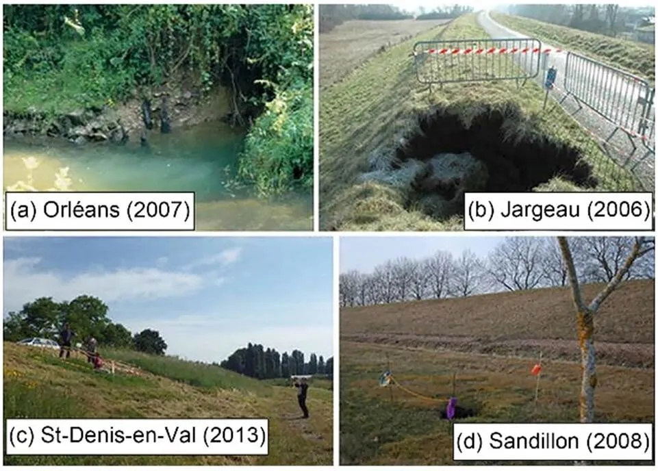
Fig. 14 Real case induced by karst existence and the geotechnical failure of some dikes in Val d'Orléans, France. The failure affects the toe (a), the head (b), and the slope face (c and d) behind the dike (Gombert et al., 2015)

The problem treated in this section is related to the stability of a dike in the presence of a soluble saturated gypsum domain which dissolves continuously in time. This dissolution is caused and sustained by a constant flow of freshwater (Fig. 15).

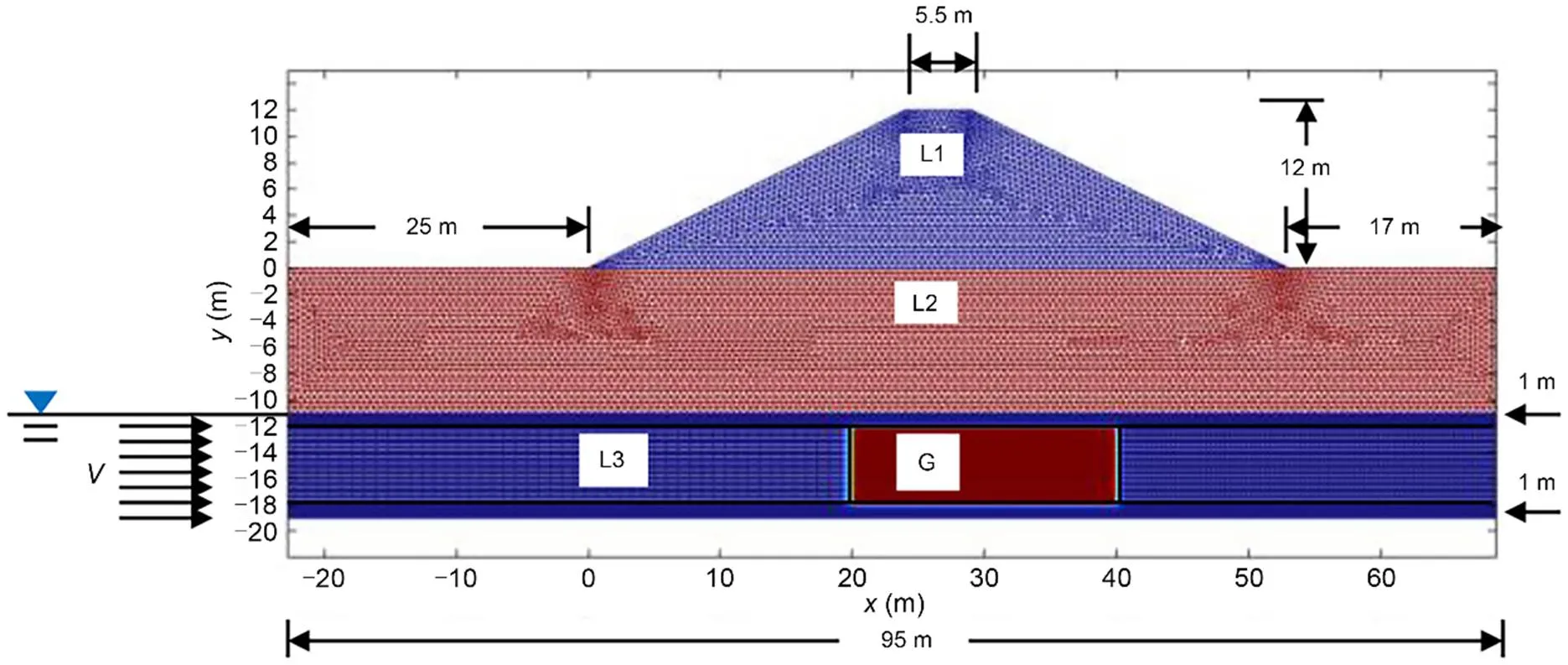
Fig. 15 Model meshed of a dike (L1): the gypsum lens (G) is located below and in the vicinity of a dike

The gypsum layer (G), 4-m thick and 20-m long (Fig. 15), is located just below an overburden (L1, L2) of (sandy-silty) soil. The gypsum domain (G) is situated in a porous medium (L3) saturated with water. Pure water thus flows at the inlet with a continuous velocityof 2.5×10-7m/s. It is supposed that the inlet concentration is zero (freshwater). A null flow condition is imposed on the lower and upper sides of the porous layer (L3) that contains the soluble part. The mechanical parameters of the soil and of the layers below the soil layer as well as those related to the dissolution are given in Table 1.

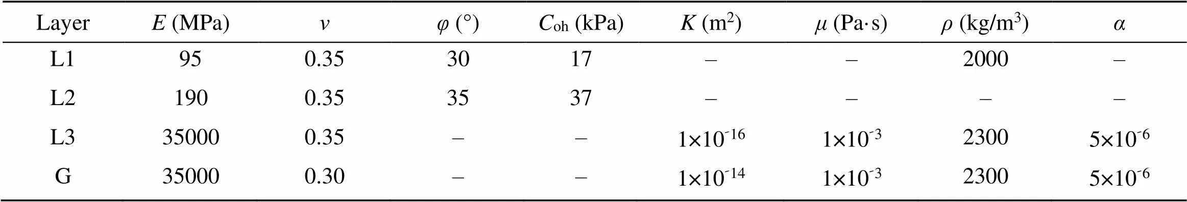
Table 1 Transport, mechanical, and dissolution parameters of the dike model

is Young's modulus,is Poisson's ratio,is the friction angle,ohis the cohesion, andis the permeability tensor

The normal displacement is imposed at all boundaries of the domain. The initial stress state is computed with gravity as the only loading. A very fine elastic (membrane) and highly deformable layer is located at the base of layer L2. The mechanical properties are such that they make it possible to dissolve a significant width without numerical instability. Indeed, when the cavity is created, the mechanisms linked to the effective collapse of the ground bell are not described in our approach. The resolution of mechanical and dissolution problems is also solved using the finite element method.

As expected, when dissolution progresses, plasticity develops in the covering soil (Figs. 16 and 17). The method provides interesting information, especially on the reduction of the stability reserve as a function of time. The knowledge of this evolution can be used for mitigation procedures and to prevent possible damage.

The maximum extension of the cavern is about 16 m at the floor and roof of the gypsum layer after 132 a. As the dissolution rate is naturally dependent on the boundary conditions, a greater flow velocity will significantly reduce this time. A rainwater inflow, for instance, can naturally create additional preferential dissolution locations within the gypsum rocks. A thorough approach that integrates the history and periodicity of soil surface rainfall is feasible with no particular problems.

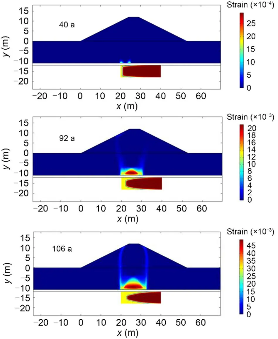
Fig. 16 Growth of the dissolution-induced cavity and the impacts in terms of soil layer plasticity (effective plastic strain) at three times: 40, 92, and 106 a (yellow represents the dissolved gypsum cavity). References to color refer to the online version of this figure

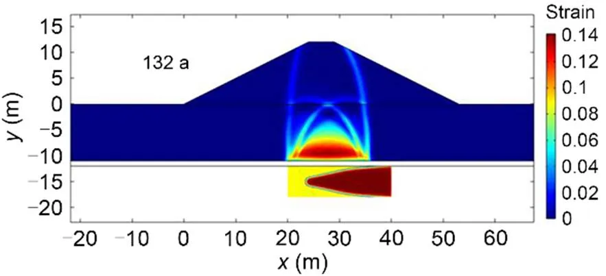
Fig. 17 Growth of the dissolution-induced cavity and the impacts in terms of soil layer plasticity (effective plastic strain) after 132 a (yellow represents the dissolved gypsum cavity). References to color refer to the online version of this figure

We observe that dissolution of the gypsum layer occurs on the boundaries which are gradually reduced. The dissolution does not occur inside the porous gypsum layer because solubility is so low that an equilibrium concentration is reached very fast.

The stability of the soil structure in our analysis is carried out with respect to a criterion of plasticity or the loss of convergence of the Newton-Raphson algorithm. More relevant criteria such as the positivity of the second order work (Hill, 1958; Prunier et al., 2009; Laouafa et al., 2011) could be used to analyze the stability.

3.2 Elastoplastic gypsum pillar dissolved at its base

In the Parisian region, the gypsum layers are very superficial. The thin overburden is not particularly resistant and is highly sensitive to the existence of caverns (Toulemont, 1987). A further issue relates to the flooding (partial or total) of gypsum mines. In certain mines, stability is provided by pillars which are left in place (Fig. 18). Their design is usually safe against many uncertainties. However, gypsum is a soluble substance and is therefore very sensitive to water. The influx of water in a continuous or periodical manner over a long period questions the effectiveness of the stability guarantee. In the short or long period of time, according to the hydraulic conditions, the pillars will lose their strength due to dissolution and the stability of the structure will be threatened.

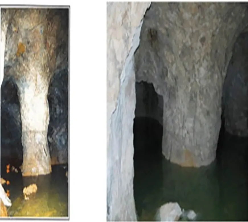
Fig. 18 Photo of pillar in the abandoned quarry with a thin layer of water at its base (by courtesy of Watelet JM, INERIS, France)

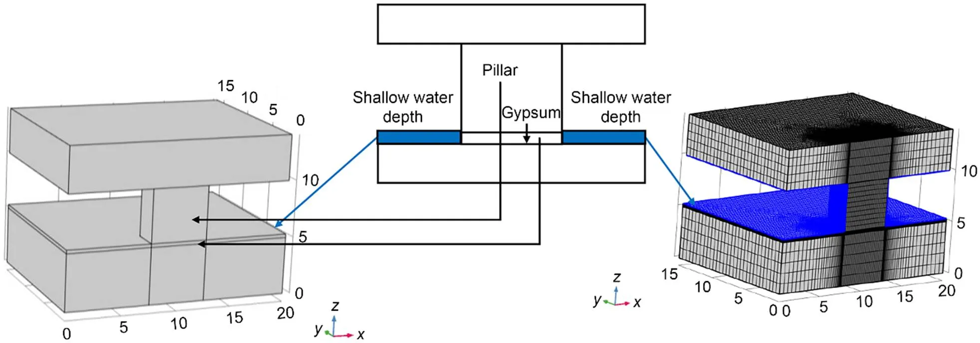
Fig. 19 Half model (left) and mesh (right) considered in computations (unit: m)

The problem of flooded mines is approached from the standpoint of the instability of a gypsum pillar that is affected by dissolution at its base by a thin layer of water. The gypsum pillar is cubic with sides of 5 m (Figs. 19 and 20). A steady flow of fresh water with zero concentration of gypsum is applied upstream. Its velocityis equal to 5×10-6m/s. The width of the water domain is 0.30 m. The thin layer of water affects only the base of the pillar. Previous calculations were performed on a cylindrically shaped pillar totally affected by water flooding. An example of state of failure is depicted in Fig. 21, showing the plasticity, after 20 a, of a cylindrical pillar subjected to continuous water flow (fluid velocity is 1×10-6m/s). The pillar is integrally submerged, and the dissolution affects all its height (Laouafa et al., 2021).

In the example below, the water dissolves the base of the cubic pillar, and computations are performed in order to analyze the plasticity or damage distribution evolving during dissolution. A dead loadequal to 450 kPa is applied on the top of the surface. The transport mechanical parameters are given in Table 2. Due to symmetries (geometry and physics), the model used in our computation is as shown in Fig. 19.

Fig. 22 shows the development of the porosity or in other terms the progress of the dissolution at four times (5, 20, 50, and 100 a). This is a bottom view of the gypsum layer. We observe a progressive loss of material and therefore of the support of the pillar with time.

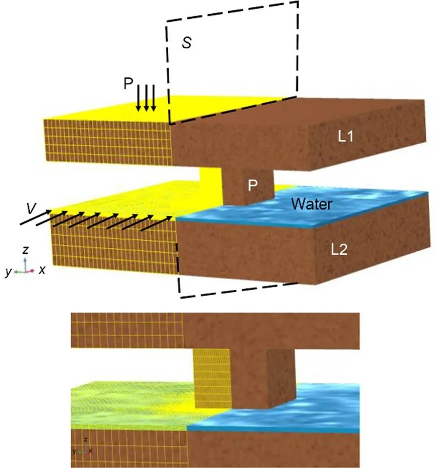
Fig. 20 Domain of the model and mechanical loading P and flow velocity V. S is a symmetry plane. Only the half domain is considered for the analysis

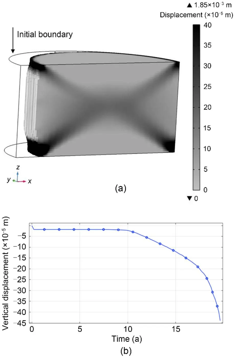
Fig. 21 Final shape and plasticity in the pillar before failure (a) and the history of the verticaldisplacement with time of a point located on the top of the pillar (b) (Laouafa et al., 2021)

The symmetry (with respect to the vertical) is preserved owing to the initial conditions. The dissolution is more severe upstream than downstream. Fig. 23 shows a 3D view of the gypsum shape lens after 100 a.

In Fig. 24 we can visualize the variation in space and for various times of the concentration of the chemical species. This description is carried out at mid thickness of the water layer. Four times are shown: 5, 20, 50, and 100 a. The normalized concentration field evolves both in intensity and in extension as dissolution progresses.

Fig. 25 shows the evolution of the effective plastic strain with the progression of dissolution. The elastoplastic pillar and the geometric configuration of the gypsum lens at different times are shown in this figure.

It is seen that dissolution of the base of the pillar leads to a concentration of stress at the boundaries of the area concerned in the dissolution. The more pronounced the dissolution is, the more the stress on the pillar increases in intensity and expands into the pillar. The distribution of plasticity and failure that can be expected is not classical.

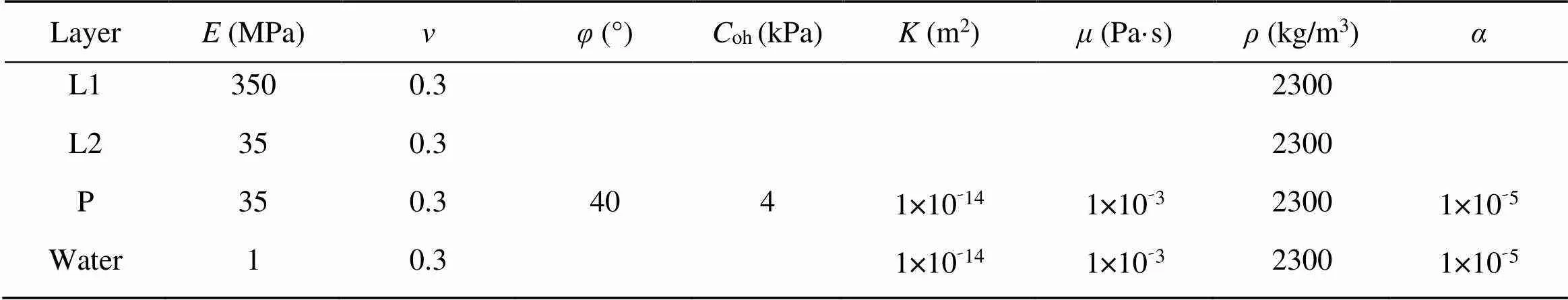
Table 2 Transport, mechanical, and dissolution parameters of the pillar model

In Fig. 26 we have only represented the plastic zones in the interior of the pillar. It is noteworthy that the effect of a thin layer of water, as compared to a total flooding, is not so common.

This is also a simple example regarding the elastoplastic model which is used to describe the behavior of gypsum material. The dissolution approach has no particular limitation on the model complexity used. Fig. 27 shows different views of the pillar deformation and the Euclidean norm of the displacement field. One can observe the loss of symmetry induced by dissolution.

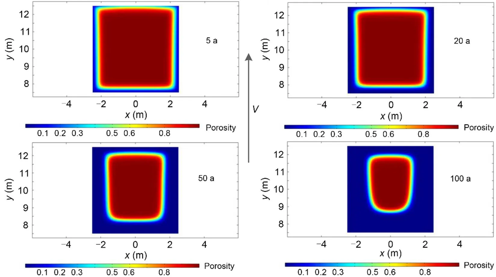
Fig. 22 Bottom view of the dissolved gypsum domain after 5, 20, 50, and 100 a (1 is solid gypsum, 0 is liquid)

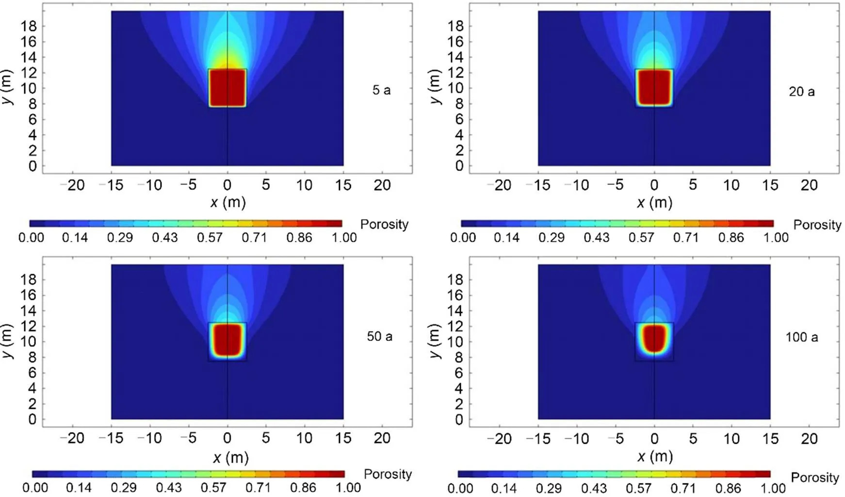
Fig. 24 Variation in space and for various times (5, 20, 50, and 100 a) of the concentration of the chemical species. Description carried out at mid thickness of the water layer

In this case, it is worth noticing that the edges of the soluble domain include geometrical singularities and the DIM method can easily circumvent them thanks to its formulation. In addition, the character of the coupling is also notable. For the same reasons as mentioned above, the dissolution does not occur in the gypsum mass but on the periphery.

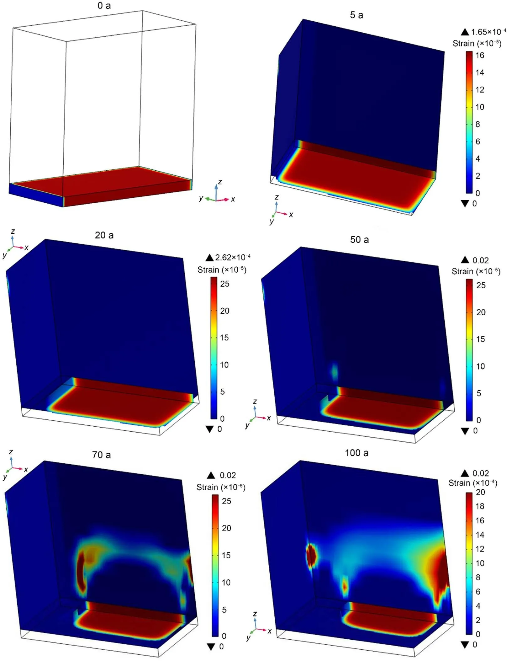
Fig. 25 Time evolution of 3D spatial distribution of effective plastic strain in 1/2 pillar at different times (0, 5, 20, 50, 70, and 100 a)

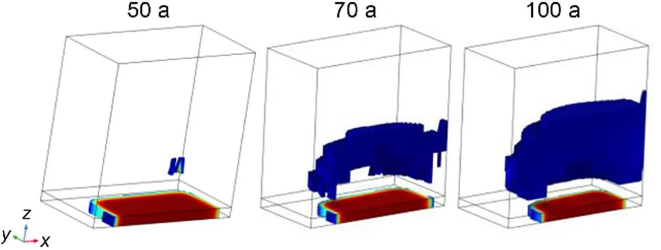
Fig. 26 Three-dimensional view of part of pillar affected by plasticity for three times (three states of dissolution)

4 Conclusions

We have discussed in this study the modeling of the dissolution of rock materials and its application in geoengineering problems. We have limited the analysis to a soluble medium that contains two phases, a porous solid phase and a liquid phase. The porous soluble medium is saturated with liquid. After the presentation of the method used to model the dissolution built on the basis of microscopic considerations and upscaling, we have applied this method in geotechnical/geomechanical applications. The issue is of noteworthy importance and the findings are very promising. The question of mid- and long-term mechanical behaviors will still arise in the presence of water in the vicinity of the evaporite present in the subsurface. The dissolution leads to a perturbation of the surroundings by the formation of voids, the modification of the morphology of structural elements, etc.

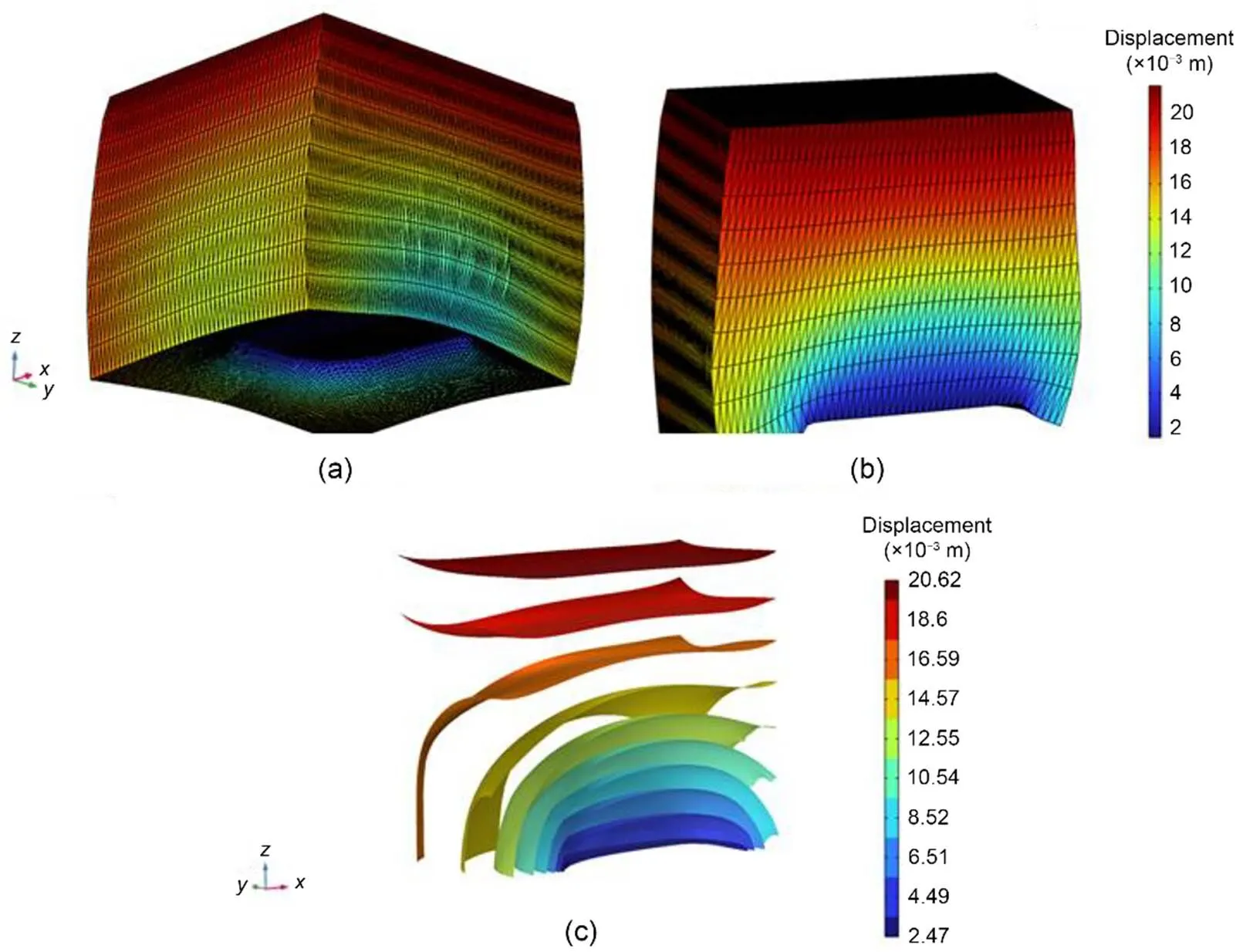
Fig. 27 Three-dimensional view (a), 1/2 model view of the Euclidean norm of the displacement (b), and 1/2 model of iso-values of the Euclidean norm of the displacement (c) (t is equal to 100 a, and magnification factors are equal to 50)

By coupling the method that describes dissolution to the geotechnical method, we explicitly introduce time (although the mechanical behavior is independent of time). It is therefore possible to foresee possible losses of stability, such as sinkholes, landslides, and failure of structures.

The developed method can be also used in the framework of underground structures like tunnels, pipelines, structures under buildings, and close to railroad tracks. Its contributions will be significant in the occurrence of an event (pipe breakage, leakage, and water intrusion).

A problem with the phenomenon of dissolution is that it is relatively slow (notably for gypsum or limestone) and the consequences are visible only in the mid or long term. Another problem is that in-situ dissolution can be only of natural origin. In such a case, we do not control all the factors (hydraulics for example). The location of the evaporites at the site scale is an additional difficulty.

In the context of such uncertainty, the proposed approach can make a meaningful contribution.

The developed approach can be extended by introducing a third phase (gas) and heterogeneities at the microscopic scale. The weak coupling in the mathematical sense can be enhanced by incorporating, for example, the evolution of the porosity induced by the deformation of the medium and by including it in the formulation of the dissolution problem.

Author contributions

Farid LAOUAFA: investigation, methodology, computation, writing-original draft, writing-review, and editing the final version. Jianwei GUO: investigation, methodology, and writing. Michel QUINTARD: investigation, writing, and validation.

Conflict of interest

Farid LAOUAFA, Jianwei GUO, and Michel QUINTARD declare that they have no relevant financial or non-financial interests to disclose.

Anderson DM, McFadden GB, 1998. Diffuse-interface methods in fluid mechanics. Annual Review of Fluid Mechanics, 30:139-165. https://doi.org/10.1146/annurev.fluid.30.1.139

Bachmat Y, Bear J, 1987. On the concept and size of a representative elementary volume (Rev). In: Bear J, Corapcioglu MY (Eds.), Advances in Transport Phenomena in Porous Media. Springer, Dordrecht, the Netherlands, p.3-20. https://doi.org/10.1007/978-94-009-3625-6_1

Bell FG, Stacey TR, Genske DD, 2000. Mining subsidence and its effect on the environment: some differing examples. Environmental Geology, 40(1-2):135-152. https://doi.org/10.1007/s002540000140

Brinkman HC, 1949. A calculation of the viscous force exerted by a flowing fluid on a dense swarm of particles. Flow, Turbulence and Combustion, 1(1):27-34. https://doi.org/10.1007/BF02120313

Castellanza R, Gerolymatou E, Nova R, 2008. An attempt to predict the failure time of abandoned mine pillars. Rock Mechanics and Rock Engineering, 41(3):377-401. https://doi.org/10.1007/s00603-007-0142-y

Charmoille A, Daupley X, 2012. Analyse et Modélisation de L’évolution Spatio-Temporelle des Cavités de Dissolution. Report DRS-12-127199-10107A, INERIS, France (in French).

Collins JB, Levine H, 1985. Diffuse interface model of diffusion-limited crystal growth. Physical Review B, 31(9):6119-6122. https://doi.org/10.1103/PhysRevB.31.6119

Cooper AH, 1988. Subsidence resulting from the dissolution of Permian gypsum in the Ripon area; its relevance to mining and water abstraction. Geological Society, London, Engineering Geology Special Publications, 5:387-390. https://doi.org/10.1144/GSL.ENG.1988.005.01.42

Donea J, Giuliani S, Halleux JP, 1982. An arbitrary Lagrangian-Eulerian finite element method for transient dynamic fluid-structure interactions. Computer Methods in Applied Mech anics and Engineering, 33(1-3):689-723. https://doi.org/10.1016/0045-7825(82)90128-1

Feng J, Hu HH, Joseph DD, 1994. Direct simulation of initial value problems for the motion of solid bodies in a Newtonian fluid. Part 2. Couette and Poiseuille flows. Journal of Fluid Mechanics, 277:271-301. https://doi.org/10.1017/S0022112094002764

Freeze RA, Cherry JA, 1979. Groundwater. Prentice Hall, Englewood Cliffs, USA, p.604.

Gerolymatou E, Nova R, 2008. An analysis of chamber filling effects on the remediation of flooded gypsum and anhydrite mines. Rock Mechanics and Rock Engineering, 41(3):403-419. https://doi.org/10.1007/s00603-007-0141-z

Gombert P, Orsat J, Mathon D, et al., 2015. Rôle des effondrements karstiques sur les désordres survenus sur les digues de Loire dans le Val D’Orleans (France). Bulletin of Engineering Geology and the Environment, 74(1):‍125-140 (in French). https://doi.org/10.1007/s10064-014-0594-8

Guo JW, Quintard M, Laouafa F, 2015. Dispersion in porous media with heterogeneous nonlinear reactions. Transport in Porous Media, 109(3):541-570. https://doi.org/10.1007/s11242-015-0535-4

Guo JW, Laouafa F, Quintard M, 2016. A theoretical and numerical framework for modeling gypsum cavity dissolution. International Journal for Numerical and Analytical Methods in Geomechanics, 40(12):1662-1689. https://doi.org/10.1002/nag.2504

Gysel M, 2002. Anhydrite dissolution phenomena: three case histories of anhydrite karst caused by water tunnel operation. Rock Mechanics and Rock Engineering, 35(1):1-21. https://doi.org/10.1007/s006030200006

Hill R, 1958. A general theory of uniqueness and stability in elastic-plastic solids. Journal of the Mechanics and Physics of Solids, 6(3):236-249. https://doi.org/10.1016/0022-5096(58)90029-2

James AN, Lupton ARR, 1978. Gypsum and anhydrite in foundations of hydraulic structures. Géotechnique, 28(3):249-272. https://doi.org/10.1680/geot.1978.28.3.249

Jeschke AA, Dreybrodt W, 2002. Dissolution rates of minerals and their relation to surface morphology. Geochimica et Cosmochimica Acta, 66(17):3055-3062. https://doi.org/10.1016/S0016-7037(02)00893-1

Jeschke AA, Vosbeck K, Dreybrodt W, 2001. Surface controlled dissolution rates of gypsum in aqueous solutions exhibit nonlinear dissolution kinetics. Geochimica et Cosmochimica Acta, 65(1):27-34. https://doi.org/10.1016/S0016-7037(00)00510-X

Ladd AJC, Szymczak P, 2021. Reactive flows in porous media: challenges in theoretical and numerical methods. Annual Review of Chemical and Biomolecular Engineering, 12:543-571. https://doi.org/10.1146/annurev-chembioeng-092920-102703

Ladd AJC, Yu L, Szymczak P, 2020. Dissolution of a cylindrical disk in Hele-Shaw flow: a conformal-mapping approach. Journal of Fluid Mechanics, 903:A46. https://doi.org/10.1017/jfm.2020.609

Laouafa F, Prunier F, Daouadji A, et al., 2011. Stability in geomechanics, experimental and numerical analyses. International Journal for Numerical and Analytical Methods in Geomechanics, 35(2):112-139. https://doi.org/10.1002/nag.996

Laouafa F, Guo JW, Quintard M, 2021. Underground rock dissolution and geomechanical issues. Rock Mechanics and Rock Engineering, 54(7):3423-3445. https://doi.org/10.1007/s00603-020-02320-y

Luo H, Laouafa F, Guo J, et al., 2014. Numerical modeling of three-phase dissolution of underground cavities using a diffuse interface model. International Journal for Numerical and Analytical Methods in Geomechanics, 38(15):1600-1616. https://doi.org/10.1002/nag.2274

Luo HS, Quintard M, Debenest G, et al., 2012. Properties of a diffuse interface model based on a porous medium theory for solid-liquid dissolution problems. Computational Geosciences, 16(4):913-932. https://doi.org/10.1007/s10596-012-9295-1

Luo HS, Laouafa F, Debenest G, et al., 2015. Large scale cavity dissolution: from the physical problem to its numerical solution. European Journal of Mechanics-B/Fluids, 52:131-146. https://doi.org/10.1016/j.euromechflu.2015.03.003

Molins S, Soulaine C, Prasianakis NI, et al., 2021. Simulation of mineral dissolution at the pore scale with evolving fluid-solid interfaces: review of approaches and benchmark problem set. Computational Geosciences, 25(4):1285-1318. https://doi.org/10.1007/s10596-019-09903-x

Prunier F, Laouafa F, Darve F, 2009. 3D bifurcation analysis in geomaterials: investigation of the second order work criterion. European Journal of Environmental and Civil Engineering, 13(2):135-147. https://doi.org/10.1080/19648189.2009.9693096

Quintard M, Whitaker S, 1994a. Convection, dispersion, and interfacial transport of contaminants: homogeneous porous media. Advances in Water Resources, 17(4):221-239. https://doi.org/10.1016/0309-1708(94)90002-7

Quintard M, Whitaker S, 1994b. Transport in ordered and disordered porous media I: the cellular average and the use of weighting functions. Transport in Porous Media, 14(2):163-177. https://doi.org/10.1007/BF00615199

Quintard M, Whitaker S, 1999. Dissolution of an immobile phase during flow in porous media. Industrial & Engineering Chemistry Research, 38(3):833-844. https://doi.org/10.1021/ie980212t

Swift G, Reddish D, 2002. Stability problems associated with an abandoned ironstone mine. Bulletin of Engineering Geology and the Environment, 61(3):227-239. https://doi.org/10.1007/s10064-001-0147-9

Toulemont M, 1981. Evolution Actuelle des Massifs Gypseux par Lessivage-Cas des Gypses Lutétiens de la Région Parisienne, France. IFSTTAR, France (in French).

Toulemont M, 1987. Les Risques D’instabilité Liés au Karst Gypseux Lutétien de la Région Parisienne‍–‍Prévision en Cartographie. IFSTTAR, France (in French).

Tryggvason G, Bunner B, Esmaeeli A, et al., 2001. A front-tracking method for the computations of multiphase flow. Journal of Computational Physics, 169(2):708-759. https://doi.org/10.1006/jcph.2001.6726

Waltham T, Bell FG, Culshaw MG, 2005. Sinkholes and Subsidence: Karst and Cavernous Rocks in Engineering and Construction. Springer, Berlin, Germany. https://doi.org/10.1007/b138363

Wang SJ, Cheng ZC, Zhang Y, et al., 2021. Unstable density-driven convection of CO2 in homogeneous and heterogeneous porous media with implications for deep saline aquifers. Water Resources Research, 57(3):e2020WR028132. https://doi.org/10.1029/2020WR028132

Whitaker S, 1999. The Method of Volume Averaging. Springer, Dordrecht, the Netherlands. https://doi.org/10.1007/978-94-017-3389-2

Yang J, Yin ZY, Laouafa F, et al., 2020. Three-dimensional hydromechanical modeling of internal erosion in dike-on-foundation. International Journal for Numerical and Analytical Methods in Geomechanics, 44(8):1200-1218. https://doi.org/10.1002/nag.3057

Mar. 28, 2022; Revision accepted July 18, 2022 Crosschecked Dec. 14, 2022

https://doi.org/10.1631/jzus.A2200169

Jianwei GUO, jianweiguo@swjtu.edu.cn

Jianwei GUO, https://orcid.org/0000-0002-0648-630X

© Zhejiang University Press 2023