Updated Simulation of Tropospheric Ozone and Its Radiative Forcing over the Globe and China Based on a Newly Developed Chemistry–Climate Model

Qi AN, Hua ZHANG, Shuyun ZHAO, Tijian WANG, Qianxia LIU, Zaizhi WANG,Sunling GONG, Bing XIE, and Yi LIU

1 Institute of Urban Meteorology, China Meteorological Administration, Beijing 100089 2 State Key Laboratory of Severe Weather, Chinese Academy of Meteorological Sciences, China Meteorological Administration, Beijing 100081 3 Department of Atmospheric Science, School of Environmental Studies, China University of Geosciences, Wuhan 430074 4 School of Atmospheric Sciences, Nanjing University, Nanjing 210023 5 CMA Earth System Modeling and Prediction Center, China Meteorological Administration (CMA), Beijing 100081 6 Key Laboratory for Climate Studies, National Climate Center, China Meteorological Administration, Beijing 100081 7 Carbon Neutrality Research Center, Institute of Atmospheric Physics, Chinese Academy of Sciences, Beijing 100029

ABSTRACT This study evaluates the performance of a newly developed atmospheric chemistry-climate model, BCCAGCM_CUACE2.0 (Beijing Climate Center Atmospheric General Circulation Model_China Meteorological Administration Unified Atmospheric Chemistry Environment) model, for determining past (2010) and future (2050) tropospheric ozone (O3) levels.The radiative forcing (RF), effective radiative forcing (ERF), and rapid adjustments (RAs,both atmospheric and cloud) due to changes in tropospheric O3 are then simulated by using the model.The results show that the model reproduces the tropospheric O3 distribution and the seasonal changes in O3 surface concentration in 2010 reasonably compared with site observations throughout China.The global annual mean burden of tropospheric O3 is simulated to have increased by 14.1 DU in 2010 relative to pre-industrial time, particularly in the Northern Hemisphere.Over the same period, tropospheric O3 burden has increased by 21.1 DU in China, with the largest increase occurring over Southeast China.Although the simulated tropospheric O3 burden exhibits a declining trend in global mean in the future, it increases over South Asia and Africa, according to the Representative Concentration Pathway (RCP) 4.5 and 8.5 scenarios.The global annual mean ERF of tropospheric O3 is estimated to be 0.25 W m−2 in 1850−2010, and it is 0.50 W m−2 over China.The corresponding atmospheric and cloud RAs caused by the increase of tropospheric O3 are estimated to be 0.02 and 0.03 W m−2, respectively.Under the RCP2.6, RCP4.5,RCP6.0, and RCP8.5 scenarios, the annual mean tropospheric O3 ERFs are projected to be 0.29 (0.24), 0.18 (0.32),0.23 (0.32), and 0.25 (0.01) W m−2 over the globe (China), respectively.

Key words: tropospheric ozone, effective radiative forcing, rapid adjustments

1.Introduction

Tropospheric ozone (O3), a major pollutant in the atmosphere, causes damage to human health and the ecosystem (Zeng et al., 2008; Stevenson et al., 2013; Lou et al., 2014, 2015; Zhu and Liao, 2016; Revell et al., 2018;Young et al., 2018).It is a prominent greenhouse gas(Zhu and Liao, 2016; Young et al., 2018) with a strong infrared absorption band at 9.6 μm (Wang, 1999; Geng et al., 2012).As such, tropospheric O3contributes significantly to the radiation budget of the earth-atmosphere system and thus has a large effect on climate.Tropospheric O3is also considered a short-lived climate forcer (SLCF),as its lifetime in the atmosphere is relatively short (Li et al., 2016; Zhang et al., 2018).Previous studies have indicated that tropospheric O3forms mainly from photochemical reactions among its precursors that include nitrogen oxides (NOx), carbon monoxide (CO), methane(CH4), and nonmethane volatile organic compounds(NMVOCs) (Stevenson et al., 2013; Liao and Shang,2015; Li et al., 2018; Revell et al., 2018).The temporal and spatial distributions of these precursors greatly affect the distribution of tropospheric O3.

Recent observations and studies have demonstrated an increasing trend in tropospheric O3, mainly in the Northern Hemisphere (NH) and especially in industrial areas.In regions with heavy industries, there has been a steady increase in O3precursor emissions from anthropogenic sources since the pre-industrial era (Logan, 1985; Volz and Kley, 1988; Ji and Qin, 1998; Wang and Sun, 1999;Lamarque et al., 2005; Stevenson et al., 2013).The steady increases in tropospheric O3precursor emissions are now having a significant effect in remote rural areas(Jacob et al., 1993; Bakwin et al., 1994).Additionally,many studies have shown a shift in high-emitting areas of anthropogenic precursors of O3from North America and Europe to Asia (Granier et al., 2011; Cooper et al., 2014;Zhang et al., 2016) and developing countries.Therefore,it is necessary to investigate changes in tropospheric O3in China and its long-term effects.

There have been numerous studies on the radiative forcing (RF) of tropospheric O3.Shindell et al.(2003)used the GISS (Goddard Institute for Space Studies)chemistry-climate general circulation model (GCM) to obtain the present global annual mean RF of tropospheric O3of 0.30 W m−2.Skeie et al.(2011) estimated an RF of 0.44 W m−2for tropospheric O3from 1850 to 2010 using OsloCTM2 (chemical transport model); additionally,their data showed an increasing trend.Søvde et al.(2011)revealed RF values of tropospheric O3and its precursors of 0.38 and 0.44 W m−2, respectively, from 1750 to 2010 with OsloCTM2.Stevenson et al.(2013) assessed the RF of tropospheric O3from 1750 to 2010 and obtained a value of 410 mW m−2with 17 atmospheric chemistry models as part of the Atmospheric Chemistry and Climate Model Intercomparison Project (ACCMIP); future tropospheric O3RF values for the year 2030 (relative to 1750) were projected to be 350, 420, 370, and 460 mW m−2under Representative Concentration Pathways(RCPs) 2.6, 4.5, 6.0, and 8.5 scenarios, respectively.Researchers have also analyzed tropospheric O3RF in China and its adjacent areas.Li et al.(2018) estimated the tropospheric O3RF as 0.69 W m−2over China and its adjacent areas in summer, which the data were obtained by using RegCM4 (Regional Climate Model version 4.0)from 2005 to 2010.Zhu and Liao (2016) estimated that the tropospheric O3RF over China was 0.48 W m−2in 2000 (relative to 1850) using GEOS-Chem (Goddard Earth Observing System-Chemistry).

The Fifth Assessment Report of the Intergovernmental Panel on Climate Change (IPCC AR5) introduced the concept of effective radiative forcing (ERF).Boucher et al.(2013) pointed out that the calculation of ERF requires longer simulations, with more complex models than that used for RF calculation; however, the inclusion of the additional rapid adjustments makes ERF a better indicator of the eventual global mean temperature response (Smith et al., 2020).Zhao et al.(2019) performed time-slice experiments to investigate the ERF of tropospheric O3with CESM1 (Community Earth System Model) and O3concentrations derived from WACCM(Whole Atmosphere Community Climate Model) simulations (Marsh et al., 2013) from 1970 to 2010; an ERF value of 0.24 ± 0.01 W m−2was obtained.Xie et al.(2016) used the BCC-AGCM_CUACE/Aero (Beijing Climate Center Atmospheric General Circulation Model_China Meteorological Administration Unified Atmospheric Chemistry Environment for Aerosols) model and off-line O3profile data from Ozone Monitoring Instrument (OMI) to calculate the global annual mean ERF of tropospheric O3; a value of 0.46 W m−2was obtained from 1850 to 2013.MacIntosh et al.(2016) estimated a tropospheric O3ERF of 0.26 W m−2using the atmosphere-only version of the HadGEM3 (Hadley Centre Global Environment Model version 3) climate model and the zonal-mean O3distribution taken from ACCMIP.However, relatively few tropospheric O3ERF studies have been performed to date, and attempts have been limited by various factors, including off-line O3data used in previous studies.In addition, some of these earlier investigations did not consider atmospheric chemistry-radiation-climate interactions (MacIntosh et al., 2016; Xie et al., 2016).As mentioned above, tropospheric O3is formed mainly by photochemical reactions; thus, it is necessary to study the ERF of tropospheric O3while considering the emissions of its precursors and chemical processes (not considering the stratosphere-troposphere transport) using a chemistry-climate online coupled model.

In this study, the tropospheric O3burden, RF, and ERF of the past are investigated in an attempt to quantify the changes in tropospheric O3and its RF and ERF for the year 2050 at global and regional scales, using our newly developed atmospheric chemistry-climate model,BCC-AGCM_CUACE2.0.Here, we focus on regions in China.

2.Methods

2.1 Model description

In this study, we simulated the burden of tropospheric O3and the associated RF and ERF due to changes in the O3burden, using the newly developed atmospheric chemistry-climate model BCC-AGCM_CUACE2.0,which couples an atmospheric GCM (BCC-AGCM2.0)and a chemistry model (CUACE2.0).

2.1.1Atmospheric general circulation model

BCC-AGCM2.0 was developed by the National Climate Center of the China Meteorological Administration(NCC/CMA; Wu et al., 2010).As part of the IPCC Coupled Model Intercomparison Project Phase 5, BCCAGCM2.0 has been validated as state-of-the-art representation against satellite observations (e.g., Zhang et al.,2012a; Jiang et al., 2015).The model adopts a horizontal resolution of 2.8° latitude × 2.8° longitude, with terrainfollowing hybrid vertical coordinates having 26 layers and a rigid lid at 2.9 hPa.Additional details, including a description of the detailed dynamics, physical processes,and validation procedure for BCC-AGCM2.0, can be found in Wu et al.(2010).The definition of tropopause in BCC_AGCM2.0 is the same as in the NCAR Community Atmosphere Model (Collins et al., 2004):

wherept(hPa) refers to the pressure at the tropopause andφrefers to latitude.

To improve the simulation of radiation fluxes at the top of atmosphere (TOA) and the surface, the cloud overlap scheme of a Monte-Carlo independent column approximation (Pincus et al., 2003; Jing and Zhang, 2012,2013) and the new Beijing Climate Center radiation transfer model (BCC_RAD; Zhang et al., 2014; Zhang,2016) were implemented.BCC_RAD divides the wavelength range (0.204-1000 μm) into 17 bands (8 longwave and 9 shortwave bands) and 5 main greenhouse gasses (H2O, CO2, O3, N2O, and CH4).In addition,three types of chlorofluorocarbons are included in the model.Gas absorption ranges and their overlaps are calculated by using the correlatedK-distribution method(Zhang et al., 2003).

2.1.2Unified atmospheric chemistry environment

CUACE2.0 is a unified atmospheric chemistry environment that includes an aerosol module (CUACE/Aero),a gas chemistry module (CUACE/Gas), and a thermodynamic equilibrium module (CUACE/ISO).CUACE/Aero is a size-segregated multicomponent aerosol module used to calculate the mass concentrations of seven aerosol species [sea salt, sand/dust, black carbon (BC), organic carbon (OC), sulfate, nitrate, and ammonium salt].The hygroscopic growth of soluble aerosol particles, such as nitrates, sulfates, OC, and sea salt, was taken into account.The performance of CUACE/Aero has been evaluated by Wang et al.(2014), Zhang et al.(2014), Wang et al.(2015), and An et al.(2019) in detail; these studies demonstrate the accuracy of this model in simulating the mass concentrations of aerosols.These information in detailed transport, physical processes, chemical transformation, cloud interactions, and the deposition of atmospheric aerosols are described in Gong et al.(2002,2003), Zhang et al.(2012b), and Zhou et al.(2012).CUACE adopts ISORROPIA to calculate the thermodynamic equilibrium between the aerosols and their gas precursors (Nenes et al., 1998; West et al., 1998; Yu et al., 2005) and is known as CUACE/ISO in our model.A more detailed description of ISORROPIA can be found in Nenes et al.(1998).

CUACE/Gas is based on the second-generation Regional Acid Deposition Model (RADM2; Stockwell et al., 1990; Zhou et al., 2012).The model consists of 63 gaseous species generated through 21 photochemical reactions and 121 gas phase reactions and is applicable under a wide variety of environmental conditions.In CUACE/Gas, OH, H2O2, O3, NO3, HNO3, and other important gas species can be simulated online.As mentioned above, NOx, CO, CH4, and NMVOCs are important precursors of O3, as they can form or consume O3(e.g., NO) through complex chemical reactions in the atmosphere.Some of the chemical reactions in which these precursors participate are described below.

Reactions (1)-(3) are fast cycle processes; the net effect of these reactions cannot promote O3formation.Reactants that can consume NO during the photolysis of NO2will be conducive to O3production; these reactants are CO, CH4, and NMVOCs.The associated reactions are given below.

CO reacts with HO to produce HO2, which can consume NO:

Combining reactions (1) and (2), the net reaction of CO to O3is as follows:

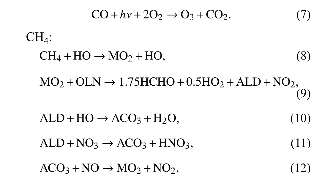
where ALD is acetaldehyde, MO2is a methyl peroxy radical, and ACO3is an acetylperoxide radical.ACO3can consume NO, which is conducive to O3formation:

NMVOCs:

Given reactions (12)-(15), the net reaction of NMVOCs to O3is given below:

where R is a hydrocarbon radical and CARB is macromolecular carbon.More detailed species, parameterization schemes, and reactions can be found in Stockwell et al.(1990).

2.2 Data and experimental design

In this study, the year 1850 was chosen to represent the O3concentration status of the pre-industrial era (PI),and the year 2010 was chosen to denote the beginning of the 21st century (BG).Choosing these particular years allowed for an RF comparison with the best estimate of RF from the IPCC AR5, in which 2010 represents the present day (PD).The year 2050 was chosen to represent the mid-term future (MT) assessment of tropospheric O3.

As mentioned above, NOx, CO, CH4, and NMVOCs are important precursors of tropospheric O3.In this study, NMVOCs include formaldehyde (HCHO), ethane(C2H6), ethylene (C2H4), isoprene (C5H8), toluene(C7H8), and xylene (C8H10), as these six species are abundant in the atmosphere and they are also the key species used in CUACE2.0.Emission data for these gases from the RCP database version 2.0 (Moss et al.,2010; van Vuuren et al., 2011) were used in our model.The emission data of O3precursors in 1850 (RCP Hist)are shown in Table 1.To investigate the variation in tropospheric O3under different emission scenarios, emission data from RCP2.6, RCP4.5, RCP6.0, and RCP8.5 for 2050 were applied.

Table 1.O3 precursor emissions in the globe and China in 1850

Table 2.Experimental design

Figures 1 and 2 show the time series of annual mean emissions of O3precursors in the globe and China from 2010 to 2050.Emissions of the four species increased significantly from 1850 to 2010, which was closely related to the large amount of anthropogenic pollutants produced after the Industrial Revolution.We also found that the anthropogenic emissions of O3precursors are much higher than the natural emissions in the future(supplement Figs.s1, s2), which means that anthropogenic emissions make a great contribution to the generation of tropospheric O3.By contrast, RCP data revealed decreasing emission trends for the four species from 2010 to 2050, indicating that tropospheric O3pollution may improve in the future.From a global perspective, it should be noted that the burden of CH4exhibits an increasing trend under RCP8.5, and CO remains basically unchanged under RCP6.0.The burden of NMVOCs exhibits a slowly increasing trend under RCP6.0; however,NOx, CO, and NMVOCs emissions in China exhibit an increasing trend under RCP6.0, significantly different from those at the global scale.This suggests that tropospheric O3pollution in China will be more severe in the near future.

In this study, six experiments are conducted (Table 2).The RF and ERF values of tropospheric O3are estimated as the differences between a specified year and the PI.Based on the emission data of the period, calculations are performed by using the BCC-AGCM_CUACE2.0 model.Sea surface temperature (SST) and sea-ice cover (SI) are fixed at values specified in 21-yr (1981−2001) climatology data from the Hadley Centre for the calculations(Hurrell et al., 2008), and the stratospheric O3is prescribed as fixed value and obtained from the OMI observational data (see http://aura.gsfc.nasa.gov/).The model integration time is 30 yr (Pincus et al., 2016; Smith et al.,2020).

Fig.1.Changes in emissions of ozone (O3) precursors from 2010 to 2050.

Observations of tropospheric O3(DU) for model validation in Section 3 are provided by the NASA’s Goddard Space Flight Center.These data with a resolution of 1.25° × 1° (valid from October 2004 to October 2010)are derived from ozone measurements obtained by OMI and Microwave Limb Sounder (MLS) onboard on theAurasatellite using the tropospheric O3residual method(Ziemke et al., 2006, 2011).These data are verified by using ozonesonde data and exhibited good reliability (Li et al., 2018).We also evaluated the performance of the model for the seasonal cycle of surface O3using data from 2014 to 2016 derived from the China National Environmental Monitoring Center (http://www.cnemc.cn/).

To calculate RF, the “double radiation call” method was used, which calls the radiation scheme twice each time step, such that the meteorological conditions remain unchanged.We used the real-time tropospheric O3concentration calculated online by the model in one call of the radiation scheme and doubled the tropospheric O3concentration in the other.During the same time step,tropospheric O3affected only the radiative process,without effect on any other climate process.RF due to tropospheric O3refers to the difference in radiative flux at the tropopause during the two calls.RF during a specified period due to tropospheric O3changes refers to the difference in RF between two time slices.The Radiative Forcing Model Intercomparison Project states that the model ERF can be diagnosed by suppressing the response, that is, by specifying SST and SI concentrations(Pincus et al., 2016).In this work, ERF values are calculated by using the method proposed by Hansen et al.(2005), which the SST and SI coverage are fixed at climatological values while allowing all other parts of the system to respond until an equilibrium state is reached.

Fig.2.As in Fig.1, but for China.

3.Validation of simulations based on 2010

Fig.3.Global distributions of tropospheric O3 (DU).(a) Simulations of BCC-AGCM_CUACE2.0, (b) observations from Ozone Monitoring Instrument (OMI)/Microwave Limb Sounder (MLS) onboard the Aura satellite, and (c) differences between simulation and observation.

Figure 3 presents the global distributions of the column concentration of tropospheric O3derived from simulations and OMI/MLS and the difference between them for 2010.BCC-AGCM_CUACE2.0 captured the tropospheric O3patterns in high-emission areas of O3precursors (mainly industrial areas), such as in North America, Middle East, South Asia, and East Asia.Simulations of the Southern Hemisphere (SH) produced values that were lower than the observations, which was mainly due to the low emissions in the SH used in this study.Moreover, the underestimates in the SH are common in most chemistry-climate models due to the inaccurate emissions (Young et al., 2013; Parrish et al., 2014;2018).Revell et al.(2018) also found that multi-model results overestimated the concentration, on average by up to 40%-50% in the NH, compared with OMI/MLS observations, and underestimated the concentrations by approximately 30% in the SH; in the study, the annual mean tropospheric column O3was analyzed by using the 15 models applied in the stratosphere-troposphere processes and their role in SPARC-IGAC (Stratosphere-troposphere Processes And their Role in Climate-International Global Atmospheric Chemistry) Chemistry-Climate Model Initiative (CCMI).Recently, Lu et al.(2020)has also developed BCC-GEOS-Chem v1.0 that can simulate the evolution of atmospheric chemical interactive constituents and capture well the spatial distributions and seasonal cycles of tropospheric O3; and this study shows that the low STE (stratosphere-troposphere exchange) in BCC-GEOS-Chem v1.0 appears to be the main factor causing ozone underestimates in the upper troposphere.

In this study, the simulated column concentration of tropospheric O3was approximately 4.9 DU lower than the observations, which is within the bias range between multi-model mean results and observations (Young et al.,2013).In addition, a different definition of tropopause in a particular model can also cause some simulation biases.However, we obtained results that are fairly consistent among regions for the tropospheric O3distribution.It should be noted that the distribution of the simulated column concentration of tropospheric O3reproduced the pattern well, compared with OMI/MLS observations for China, with a difference in the annual mean value of only 0.1 DU (Fig.4).The lower simulation values for the Qinghai-Tibetan Plateau were mainly due to the fact that the model did not consider O3stratosphere-troposphere transport.

Fig.4.As in Fig.3, but for China.

To further evaluate the performance of the model for the seasonal cycle of surface O3in China, we first divided China into the following five geographic areas:Northeast China (NEC; 38°-55°N, 121°-135°E), North China (NC; 33°-50°N, 110°-121°E), Northwest China(NWC; 34°-50°N, 73°-110°E), Southwest China (SWC;21°-34°N, 78°-110°E), and Southeast China (SEC;17°-33°N, 110°-123°E).In each area, surface O3concentrations were observed from four sites distributed evenly throughout the area; the sites are shown in Fig.5(blue dots).The observations showed that the maximum surface O3concentrations occurred during the summer,whereas the minimum concentrations occurred during the winter in most areas (Fig.6).This is mainly due to the strong sunlight and high temperatures in summer, which are conducive to O3formation.By interpolating the simulations over the observation site using bilinear interpolation, we found that the simulated surface O3concentrations matched the seasonal evolution of the observed concentrations in China well, although some sites showed a slight bias.The small bias in NEC might have been brought about by the emission data (An et al.,2019).This indicates that extensive efforts are still required to improve emission data and simulations in future studies.In addition, the model resolution and method of interpolation can also introduce some biases between simulations and observations (Wild and Prather, 2006;Hodnebrog et al., 2011; Stock et al., 2014).The simulated surface O3concentrations were lower than the observations during spring in Lhasa, which is mainly due to the high altitude of Lhasa; thus, the downward transport of O3from the stratosphere can have a great influence on surface O3concentration.Notably, we did not consider the O3transported via stratosphere-troposphere transport, which might have resulted in an underestimation for Lhasa.However, the simulations captured the seasonal cycle at most sites in China well.Therefore, overall, our results demonstrate that the BCC-AGCM_CUACE2.0 model can reasonably reproduce the distribution and annual mean value of tropospheric O3globally and for China.As such, we applied the model to further analyze the RF and ERF of tropospheric O3.

Fig.5.Distribution of observation sites in China.

4.Column burden of tropospheric O3

Figure 7 shows the changes in O3precursor emissions from 1850 to 2010, with areas with high concentrations of NOxand CO located mainly in eastern North America,Europe, and eastern China (Fig.7a).The East USA,Southeast Asia (especially Malaysia and Indonesia), Indian Peninsula (especially northern India), and East China emit large amounts of CO, which is closely related to local industrial and domestic emissions.Most high-CH4areas were located in northern India, Malaysia, NC, and SWC.Compared with NOx, CO, and CH4, the magnitudes of increased NMVOCs were larger and their distribution coverage more widely spread.Besides the industrial areas, NMVOCs also exhibited substantial increases over the central part of South America and the central part of southern Africa, which is mainly due to biogenic VOCs (BVOCs) such as isoprene.

The simulated global annual column burden of tropospheric O3increased by 14.1 DU from the PI to the BG,with the greatest increase in tropospheric O3over the industrialized NH, including China, India, Southeast Asia,and the Arabian Peninsula (Fig.8a).The value of tropospheric O3over China increased by approximately 21.1 DU, which is much higher than the global annual mean value.For China, the greatest increase in tropospheric O3is located over SEC and some parts of SWC; in this case,the increase is closely related to O3precursor emissions.Additionally, lower O3precursor emission is the main cause for the low column burden of tropospheric O3over the Tibetan Plateau; here, a higher altitude and lower tropopause are the two main contributing factors.

Table 3 compares calculated changes in the column burden of tropospheric O3from the PI to the BG in this work with those reported by other studies.The value obtained in this study is close to the multi-model mean value of Gauss et al.(2003), but 2.7 DU higher than the value cited by Skeie et al.(2011).This is because Skeie et al.(2011) used the BVOCs emissions in 2000 to represent the emissions in 2010 in their study, which might have introduced some underestimation.The value in Xie et al.(2016) is much higher, using off-line O3profile data from OMI in 2013; thus, the interaction between radiation and O3chemistry was not considered in their simulation.In addition, different definitions of the tropopause may also explain the discrepancies among the abovementioned study results (Young et al., 2013).

Table 3.Comparison of increased tropospheric O3 (DU) from the PI to the BG in this study with the results of other studies

Fig.6.Seasonal cycles of simulations (interpolated over observation sites) and observations from the China National Environmental Monitoring Center of surface O3 concentration (ppbv) in China.The blue curves are the simulated values for 2010.The red curves are the mean observation values from 2014 to 2016.

With the reduction of precursor emissions, global tropospheric O3is predicted to decline under different scenarios in 2050 (Fig.9).The global annual mean column burden of tropospheric O3is predicted to decrease by 2.28, 1.23, 2.49, and 0.30 DU by 2050 (relative to 2010)under RCP2.6, RCP4.5, RCP6.0, and RCP8.5, respectively.The largest reduction, 11%, occurs under RCP6.0.It should be noted that tropospheric O3is predicted to increase over India and some parts of Africa under RCP4.5 and RCP8.5.Especially over India, the maximum increase in tropospheric O3is expected to exceed 4 DU.Over Africa, the area of tropospheric O3increase is broader under RCP8.5, which may be related to the large amount of BVOCs emissions locally.From Fig.1, we can see that global CH4emissions exhibit an obvious increasing trend, whereas NMVOCs emissions remain nearly unchanged; this may explain why global tropospheric O3does not decrease significantly under RCP8.5.For China, the largest reduction in tropospheric O3occurs under RCP2.6, with an annual mean value of 3.97 DU by 2050 (relative to 2010), which would be 12.6%lower than the level in 2010, especially over NC and SEC (Fig.10).The annual mean value of tropospheric O3is predicted to decrease by 2.28 DU (7.3%) by 2050.However, a positive value is predicted for the Qinghai-Tibet Plateau, mainly due to the transportation of high concentrations of O3from northeast India.Similarly,SWC will also be affected by high concentrations of O3from northeast India under RCP8.5, resulting in an increase of 1.05 DU of tropospheric O3by 2050.In addition, NC will likely see a slight increase in tropospheric O3over the same period.

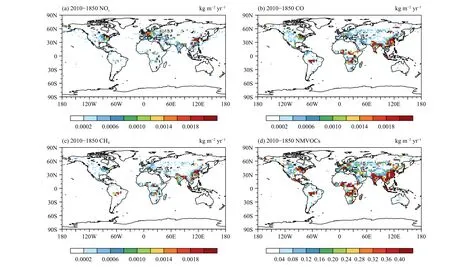
Fig.7.Distributions of O3 precursors (kg m−2 yr−1) in 2010 (relative to 1850).

Fig.8.Distributions of tropospheric O3 (DU) over (a) the globe and (b) China in 2010 (relative to 1850).

5.Radiative forcing of tropospheric O3

Figure 11 presents the global distribution of tropospheric O3RF at the tropopause at the BG relative to the PI.The RF distribution pattern is basically consistent with the distribution of tropospheric O3column burden,such that high values appear over China, India, and Southeast Asia.Thus, this suggests that tropospheric O3is the main factor affecting the magnitude of RF.The global annual mean RF value of tropospheric O3was 0.48 W m−2, within the estimation range reported in IPCC AR5 of 0.4 (0.2-0.6) W m−2(Boucher et al., 2013)and IPCC AR6 of 0.47 (0.24-0.70) W m−2(Forster et al.,2021).The normalized RF (NRF) of tropospheric O3was 34 mW m−2, which is very close to the value of 36 mW m−2obtained by Gauss et al.(2003) using multi-model results (Table 4).

The annual mean RF of tropospheric O3over China was 0.59 W m−2.Higher values appeared over SEC (0.76 W m−2) and NC (0.62 W m−2), followed by NEC, NWC,and SWC (0.56, 0.56, and 0.57 W m−2, respectively).Table 5 compares the RF values in this work with those of other studies.

Corresponding to the changes in tropospheric O3burden, global tropospheric O3RF is predicted to decline in 2050 relative to 2010, and the RF distributions are predicted to be similar among the four scenarios, as shown in Fig.12.The projected global annual mean values of tropospheric O3RF are 0.42, 0.45, 0.41, and 0.47 W m−2in 2050 under the RCP2.6, RCP4.5, RCP6.0, and RCP8.5 scenarios relative to the PI, respectively (Table 6).The O3RFs for 2050 are expected to decrease by 12.5%,6.3%, 14.6%, and 2.1% relative to 2010 under RCP2.6,RCP4.5, RCP6.0, and RCP8.5, respectively.The largest reduction in RF occurs under RCP6.0, with a value of−0.07 W m−2.The annual mean tropospheric O3RF over China is predicted to decrease by 0.08, 0.03, and 0.04 W m−2under RCP2.6, RCP4.5, and RCP6.0 from 2010 to 2050, respectively (Fig.13).It should be noted that RF is estimated to increase by 0.01 W m−2under RCP8.5, consistent with the changes in the burden of tropospheric O3.

Table 4.Comparison of the column burden, RF, and NRF of tropospheric O3 in this work and other works from the PI to the BG

Table 5.Comparison of simulated annual mean tropospheric O3 RF (W m−2) in this work and other works in the globe and China for the BG relative to the PI

Table 6.Annual mean tropospheric O3 RF (W m−2) in 2050 relative to the PI (values in brackets are changes relative to 2010)

6.Effective radiative forcing

6.1 Effective radiative forcing of tropospheric O3

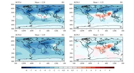
Fig.9.Global distributions of tropospheric O3 (DU) under different scenarios in 2050 (relative to 2010).

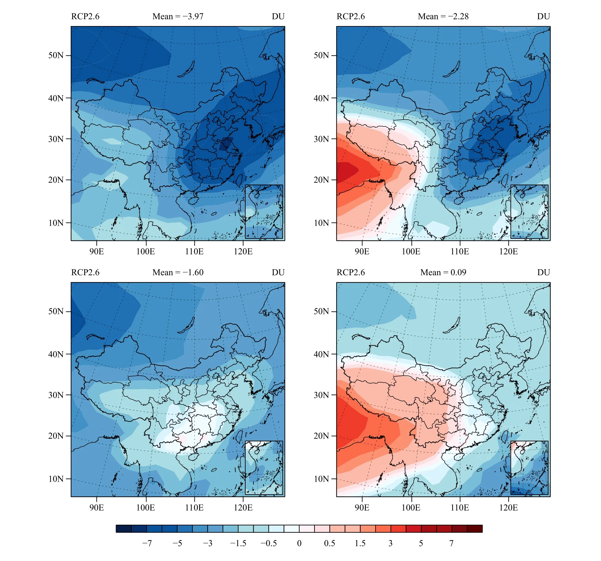
Fig.10.As in Fig.9, but for China.

Boucher et al.(2013) in IPCC AR5 proposed the ERF concept, stating that it is a better indicator of the eventual global mean temperature response.Our results show that the ERF is evenly distributed, with no obvious patterns(not closely correlated with the change in burden of tropospheric O3), and many places are associated with negative values (Fig.14).Thus, the discussion focuses on annual mean values (Zhang et al., 2018).The global annual mean ERF of tropospheric O3is 0.25 W m−2in 2010 relative to the PI (Fig.14), which is close to the value of 0.26 W m−2calculated by MacIntosh et al.(2016).The annual mean ERF value of tropospheric O3over China is 0.50 W m−2, twice the global mean value, indicating that the effect of tropospheric O3is significant for China.Although the ERF distribution exhibits no obvious patterns and is positive in many places, ERF values still have some dependence on cloud distribution.Figure 15 indicates that positive ERF values occur where the total cloud cover (TCC) is reduced, such as over western Europe,southern Australia, NEC, and SEC.Meanwhile, negative values are obtained in areas where TCC increases, e.g.,over the East European Plain, India, and SWC.This is because rapid adjustments of cloud cover can significantly affect local radiation flux (Takemura et al., 2002;Zhang et al., 2012a; An et al., 2019).

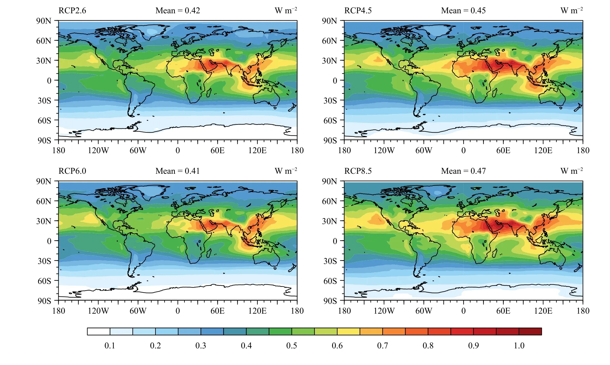
Fig.12.Global distributions of tropospheric O3 RF (W m−2) at the tropopause in 2050 (relative to the PI).

Fig.13.As in Fig.12, but for China.

To further investigate the impact of cloud cover on ERF values, the relationship between changes in longwave ERF (LW ERF) and changes in high cloud cover(HCC) from the PI to the PD are investigated (Fig.16),as well as the relationship between changes in shortwave ERF (SW ERF) and changes in low cloud cover (LCC)(Fig.17).Figure 16 shows that LW ERF is positive with increased HCC over northern South America, Europe,Central Africa, South Asia, and SWC.This is because an increase in HCC leads to greater absorption of LWR (Liu and Ye, 1991; Lelli et al., 2014), thus reducing outgoing longwave radiation at the TOA and resulting in a positive shift in LW ERF.More LWR will be emitted from the TOA in areas where the cloud cover is reduced, resulting in enhanced negative LW ERF values.Thus, negative LW ERF values appeared with a reduction in HCC over parts of the United States, the Arabian Peninsula,Australia, NWC, and SEC.Conversely, an increase in LCC leads to additional reflection of shortwave radiation out of the TOA due to the increased albedo, which enhances negative SW ERF values.Less shortwave radiation is emitted from the TOA in areas where there is less LCC, resulting in a positive shift in SW ERF values.Hence, areas with more LCC were associated with negative SW ERF values, such as over the northern part of South America, the Arabian Peninsula, South Asia,Southeast Asia, and SWC; areas with less LCC were associated with positive SW ERF, such as over the northeast part of South America, northern Africa, East China,and SEC.

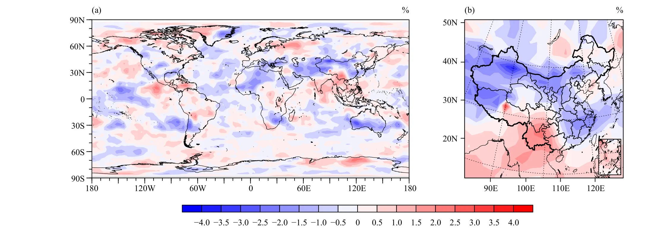
Fig.15.Distributions of clouds (%) over (a) the globe and (b) China in 2010 (relative to the PI).

Table 7 compares current studies on tropospheric O3ERF.The ERF value of the current study is very close to that of MacIntosh et al.(2016), but much smaller than that given by Xie et al.(2016).It should be noted that Xie et al.(2016) used off-line O3profile data from OMI observations; in this case, there may be contributions from the stratosphere.In addition, feedback between chemical processes and the climate in Xie et al.(2016)was not considered.In contrast to the earlier studies, our model calculates only tropospheric O3formed by chemical reactions due to its precursors; thus, the transportation of O3from the stratosphere is not a contributing factor.

Future global annual mean ERF values of tropospheric O3were predicted to be 0.29, 0.18, 0.23, and 0.25 W m−2under RCP2.6, RCP4.5, RCP6.0, and RCP8.5 in 2050, respectively.As for China, the corresponding values were 0.24, 0.32, 0.03, and 0.01 W m−2for the year 2050, respectively.Table 8 shows the changes in the ERF of tropospheric O3for 2050 relative to 2010.With the implementation of pollutant reduction measures(Huang, 2006; Zhu and Liao, 2016; Saikawa et al., 2017;Geng et al., 2019), the ERF of tropospheric O3over China is projected to decrease significantly in the future.

Fig.16.Distributions of tropospheric O3 longwave ERF (top row; W m−2) and high cloud cover (bottom row; %) over the globe and China in 2010 (relative to the PI).

6.2 Rapid adjustments in effective radiative forcing

Chung and Soden (2015a, b) pointed out that ERF is composed of RF and rapid adjustments (RAs).RAs can be further divided into RAs of the atmosphere (RAatm)and RAs of clouds (RAcld) (Smith et al., 2018, 2020;Zhao and Suzuki, 2019).In this section, the RF and ERF values refer to changes in the net radiation flux at the TOA caused by tropospheric O3(unless specified, the calculation of the radiation process is under all-sky conditions in this work).According to IPCC AR5 (Boucher et al., 2013), RAs caused by a forcing agent (here, tropospheric O3) can be obtained by subtracting its RF from the corresponding ERF.RAatmcan be obtained by using the same approach as that for determining RAs; however,clear-sky conditions are applied (i.e., the residual of ERFclrand RFclrin which the subscript “clr” refers to clear-sky conditions).RAcldis determined based on the residuals of RA and RAatm.An RA flowchart for the calculations is provided by Zhao and Suzuki (2019).

Table 9 shows the global annual mean tropospheric O3values of ERF, RF, and their differences (namely, RAs)at the TOA in 2010 relative to the PI.The total RAs(RAtot) can be expressed as

which is 0.05 W m−2.RAatmcan be expressed as

with the value of 0.02 W m−2.Thus, RAcldcan be calculated as

producing a value of 0.03 W m−2.Table 10 lists the RAatmand RAcldvalues due to tropospheric O3for the year 2050 relative to the PI.The largest RAcldof 0.07 W m−2is obtained under RCP2.6.

Table 7.Comparisons of the simulated annual mean tropospheric O3 ERF (W m−2) in this work and in other works for the BG relative to the PI

Table 8.Change in annual mean ERF value (W m−2) of tropospheric O3 in 2050 relative to 2010

Table 9.Global annual mean tropospheric O3 ERF, RF, and their difference (W m−2) at the TOA in 2010 relative to the PI.

Table 10.RAs due to tropospheric O3 in 2050 relative to the PI (W m−2).

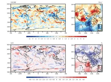
Fig.17.Distributions of tropospheric O3 shortwave ERF (top row; W m−2) and low cloud cover (bottom row; %) over the globe and China in 2010 (relative to the PI).

7.Conclusions

In this study, a newly developed atmosphere chemistry-climate model, BCC-AGCM_CUACE2.0, was used to simulate the past and future burden, RF, and ERF of tropospheric O3, and the corresponding RA for the atmosphere (RAatm) and clouds (RAcld).The model reproduced the geographical distribution and seasonal changes in tropospheric O3well, especially over China.However,biases might have been introduced by inaccuracies in the emission inventory of the SH compared with the observations derived from OMI/MLS, which is a common problem in current chemistry-climate models, as pointed out by Young et al.(2013).

The global annual mean burden of tropospheric O3was predicted to have increased by 14.1 DU from the PI to 2010, with China, South Asia, and the Arabian Peninsula seeing more significant increases.As a high-emission area in 2010, the burden of tropospheric O3over China increased by as much as 21.1 DU, with the largest value of 32.2 DU occurring over SEC.By 2050, global tropospheric O3is expected to decrease by 0.30-2.49 DU globally compared with 2010 levels, whereas the corresponding burden over China should decrease by 3.97,2.28, and 1.60 DU under the RCP2.6, RCP4.5, and RCP6.0 scenarios, respectively.However, tropospheric O3over China exhibited a different trend under RCP8.5,with its burden predicted to increase by 0.09 DU, which may be due to the influence of a high tropospheric O3burden over South Asia.

The annual mean tropospheric O3RF between the PI and the BG at the tropopause was estimated to be 0.48 globally and 0.59 W m−2over China.The RF distribution was consistent with the distribution of the column burden of tropospheric O3.With a reduction in tropospheric O3, the global annual mean RF value was predicted to be 0.41-0.47 W m−2according to different scenarios by 2050, whereas the RF over China was expected to reach 0.51-0.60 W m−2; thus, China will still experience severe ozone pollution in the future.

The global annual mean ERF for tropospheric O3at the TOA was estimated to be 0.25 W m−2for the year 2010.Meanwhile, the RAs of atmosphere and clouds were 0.02 and 0.03 W m−2, respectively.By 2050, global ERF values are expected to reach 0.29, 0.18, 0.23, and 0.25 W m−2under the RCP2.6, RCP4.5, RCP6.0, and RCP8.0 scenarios, respectively.As for the ERF over China, an estimate of 0.50 W m−2was obtained for 2010,with lower values of 0.24, 0.32, 0.03, and 0.01 W m−2by 2050.The ERF distribution was consistent with the cloud cover distribution.Positive (negative) ERF occurred in areas with an increase (decrease) in HCC.In addition, an increase in LCC can cause a negative shift in ERF, and vice versa.

Additionally, we will validate our simulation of O3concentration in other areas outside China by getting higher resolution observational data in the future.

Acknowledgments.We thank the anonymous reviewers and editors for their valuable and stimulating comments, which have greatly improved our paper.