NO-ARBITRAGE SYMMETRIES*

Iv´an DEGANO

Departamento de Matem´atica. Facultad de Ciencias Exactas y Naturales， Universidad Nacional de Mar del Plata. CONICET. Funes 3350， Mar del Plata 7600， Argentina E-mail: ivandegano@mdp.edu.ar

Sebasti´an FERRANDO†

Department of Mathematics， Ryerson University， 350 Victoria St.， Toronto， Ontario M5B 2K3，Canada E-mail: ferrando@ryerson.ca

Alfredo GONZ´ALEZ

Departamento de Matem´atica. Facultad de Ciencias Exactas y Naturales， Universidad Nacional de Mar del Plata. Funes 3350， Mar del Plata 7600， Argentina E-mail: algonzal@mdp.edu.ar

Abstract The no-arbitrage property is widely accepted to be a centerpiece of modern financial mathematics and could be considered to be a financial law applicable to a large class of (idealized) markets. This paper addresses the following basic question: can one characterize the class of transformations that leave the law of no-arbitrage invariant? We provide a geometric formalization of this question in a non probabilistic setting of discrete time-the so-called trajectorial models. The paper then characterizes， in a local sense， the no-arbitrage symmetries and illustrates their meaning with a detailed example. Our context makes the result available to the stochastic setting as a special case.

Key words No arbitrage symmetry; convexity preserving maps; non-probabilistic markets

1 Introduction

The principle of no-arbitrage plays a fundamental role in modern financial mathematics;see[11]and references therein(we mostly restrict our comments and developments to a discrete time setting). In plain language， the assumption of no-arbitrage means that risky asset models should rule out a priori the possibility of making a profit without taking on any risk. This hypothesis implies a pricing methodology based on martingale stochastic processes; this is the risk-neutral valuation([2])， and as such plays the role of a financial law. The empirical validity of this law has been studied([14])and even if arbitrage opportunities may be available，they are believed to be rare， short lived and hard to profit from. One could compare the notion of noarbitrage to a physical law(such as the principle of inertia)that applies in idealized conditions，and think of it as a fundamental financial law applicable to a large class of(idealized)markets.With this point of view in mind， and as a preliminary step， we pose the question: can we characterize the class of transformations that leave the law of no-arbitrage invariant? This is much akin to Galilean/Lorentz transformations leaving the class of inertial frames invariant.Therefore，we look for no-arbitrage preserving transformations(referred to also as no-arbitrage symmetries) mapping a set of financial events into another set of financial events with the property that the no-arbitrage property holds for both classes of events. We are also interested in providing a financial interpretation to such a set of symmetries (much like Galilean/Lorentz transformations having a physical interpretation) and exploring some financial implications.

The financial events mentioned in the previous paragraph have to be linked to financial transactions， as it is the latter that fall under the scope of the no-arbitrage principle. In most situations， each such transaction involves two goods， X and Y， and a price XY(t)， so that X =XY(t)Y. XY(t) is the integer number of units of asset Y required to purchase one unit of asset X. In terms of dimensional units， [XY(t)] =[X]/[Y]， and the reference asset Y is called the (chosen) numeraire ([19]). This discussion suggests that an analysis of the no-arbitrage principle could be done in terms of prices and numeraires (numeraire free approaches are also possible)， and that is the way we proceed in the paper.

The setting in which we precisely pose and answer the above raised question is a set of sequences of multidimensional prices that evolve in discrete time. This type of set is called a trajectorial model (for a set of risky assets); in our investigation there is no need to assume any probability structure on such a set. In this way we can work on a more general setting than the (discrete time) stochastic framework and the question we study becomes a natural one unencumbered by unnecessary additional structure. We also briefly indicate how our main results， characterizing no-arbitrage transformations，apply to the stochastic setting as a special case.

The above-mentioned trajectorial framework has been developed in [9] and [6] (see also[10]) for the 1-dimensional case with a 0% interest rate bank account as numeraire and is here extended to the d-dimensional case and a general numeraire (but we restrict ourselves to finite time， as opposed to unbounded or infinite discrete time as in[9]and[10]，respectively). It then follows that the global notion of no-arbitrage， i.e. involving several time steps， can be reduced to the one step notion of no-arbitrage. This is a classical reduction in discrete and finite time and allows us to concentrate our efforts on the local notion (i.e. involving one step into the future) of no-arbitrage.

We can now be more precise about our search for no-arbitrage preserving transformations.

We prove in this paper (by means of Proposition 4.2， Proposition 3.5 and Definition 3.6)that the notion of a set being disperse is equivalent to the risky assets(one step time evolution)obeying the no-arbitrage principle. Therefore， our original question on no-arbitrage preserving transformations turns into the challenge of characterizing the set of transformations that leave the disperse property invariant. We are then in the context of a modern view of a geometry where we study the set of transformations that leave certain properties of a space of points invariant. Lemma 4.7 shows， at the geometric level， how disperse sets are transformed under Strict Inverse Convexity Preserving (SICP) maps. Theorem 5.4 and Corollary 5.6 make use of this connection relying on the financial interpretation， where coordinates are discounted in units of a numeraire.

We work on a self contained framework for financial markets centered on a set of (mutidimensional) trajectories modeling a collection of assets with the possibility that any of them could play the role of a numeraire asset. No probability measures， filtrations， cardinality or topological assumptions are required of the trajectory set. The approach singles out local trajectory properties that can be used to consistently build an associated option price theory. The paper does not pursue this latter possibility， as we focus on symmetry transformations(option pricing developments are in [9] for the 1-dimensional case). Such trajectory properties have already made their appearance in the stochastic literature ([1， 5， 12]). To relate to the wellestablished stochastic approach ([11])， the reader could think that our paper concentrates on financial developments that only depend on the support of a given stochastic process independently of any possible probability distribution. Some connections with the stochastic setting are developed in[9];the reference[10]provides a first mathematical step to extend some martingale notions from the standard setting to a trajectorial setting.

The subject of the paper is the study of fundamental symmetry transformations associated to the no-arbitrage principle in a non-probabilistic setting. Results are obtained with minimal assumptions and， in this way， provide a wider financial context for their availability.

We now describe the contents of the paper. Section 2 introduces the setting， which is centered on a trajectory space. Section 3 studies the notions of no-arbitrage and 0-neutrality(a weakening of no-arbitrage) in trajectory based markets. Subsection 3.1 introduces local conditions (i.e. properties that are conditioned on a given state of affairs and involve one step into the future) which are necessary and sufficient to establish no-arbitrage and 0-neutrality.These local conditions play a role analogous to that of the martingale condition in stochastic markets. Section 4 develops purely geometric results in Rd，independent of any financial setting，that form the backbone for deriving the set of no-arbitrage and 0-neutral symmetries. Section 5 characterizes two classes of transformations， one preserving the local no-arbitrage property and the other class preserving the 0-neutral property. In particular， we prove that a change of numeraire belongs to both such classes of transformations. The uncovered transformations can then be considered to be symmetries satisfied by price relationships. This latter point of view is carefully developed in an example in Section 6. Appendix A.1 provides proofs for results in the main body of the paper. Appendix A.2 develops some results on convex analysis that we rely upon. Finally， it should be noted that we use the words arbitrage-free and no-arbitrage interchangeably.

2 General Trajectorial Setting

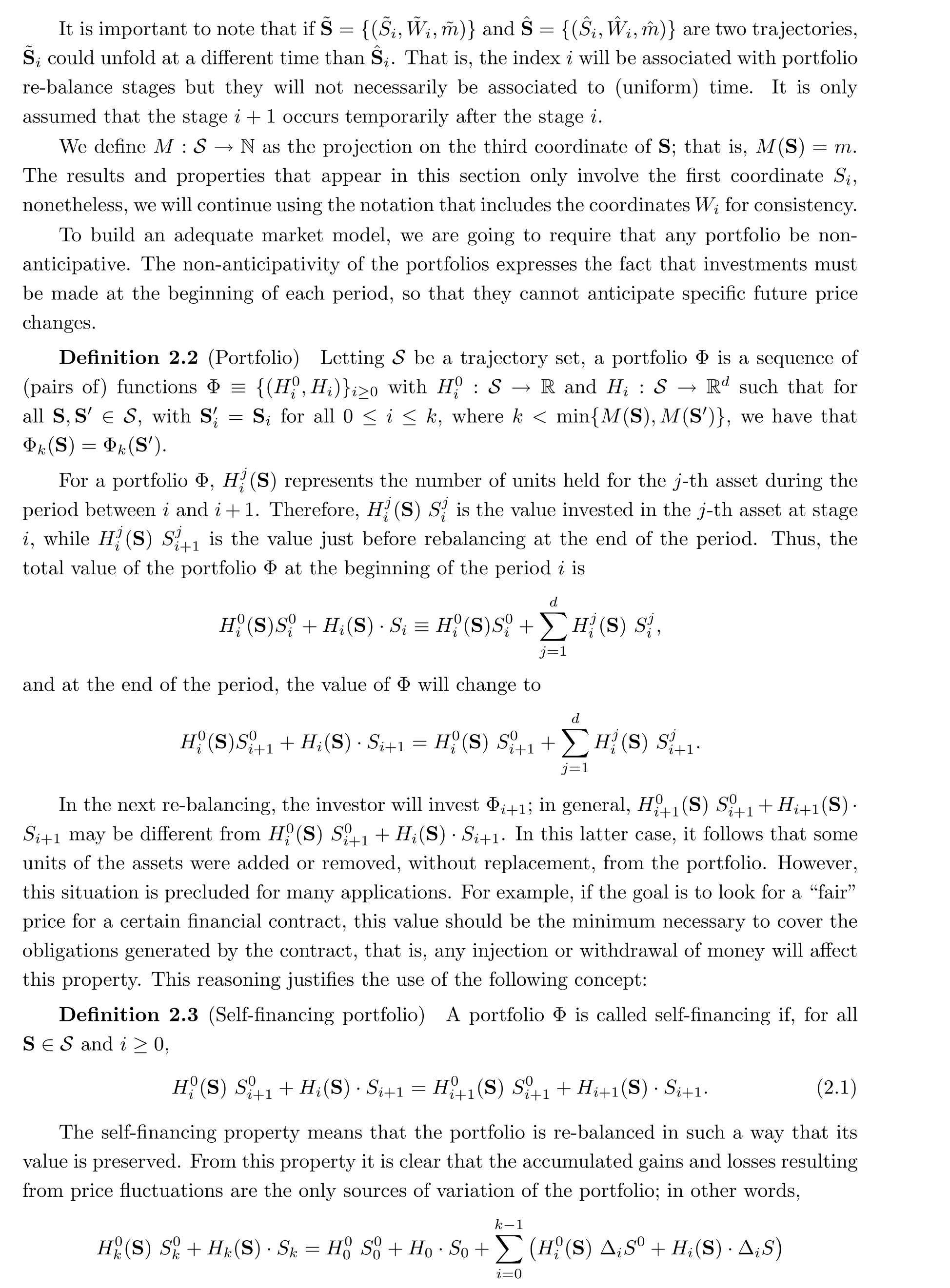
We introduce the mathematical setting of a dynamic financial market with a finite number of assets whose initial prices are known. Uncertainty of future prices is given by a set of multidimensional sequences that we call trajectories. The trading strategies are given by portfolios that will be successively re-adjusted，taking into account the information available at each stage. The present paper is essentially self-contained， though we extend work presented in [6]and[9]. The latter reference presents a non-probabilistic，one-dimensional，discrete time setting to price European options. The reference[6] provides examples and a computational algorithm to evaluate price bounds for European options. A detailed discussion and justification of why a trajectorial modeling approach is worth studying is presented in [9] as well as in [6]. The present paper extends the setting from those two papers to the multidimensional case.

The portfolio re-balancing stages may be triggered by arbitrary events of the market without the need to be directly associated with time. To incorporate this greater degree of generality we will add a new source of uncertainty to the trajectories’coordinates(these additional coordinates are relevant when constructing specific models); we will denote them by W ={Wi}i≥0， where the Wican be vector valued and take values in arbitrary sets. In financial terms， this new variable can represent any observable value of interest， such as volume of transactions， time，quadratic variation of trajectories， etc.， as in [8].

In case one intends to price financial derivatives in the proposed setting， we add a finite time horizon T. We will use a positive integer m to indicate the stage at which the trajectory reaches the time T. This new variable plays a key role in calculating the fair price interval for options， although it does not intervene in the market properties.

Definition 2.1 (Trajectory set) Consider Σ = {Σi} to be a given family of subsets of Rd+1， Ω = {Ωi} a family of sets and Θ ⊆N. For given s0∈Rd+1and w0∈Ω0， a trajectory based set S is a subset of

such that (S0，W0)=(s0，w0). The elements of S will be called trajectories.

2.1 Numeraire

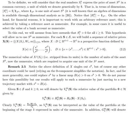
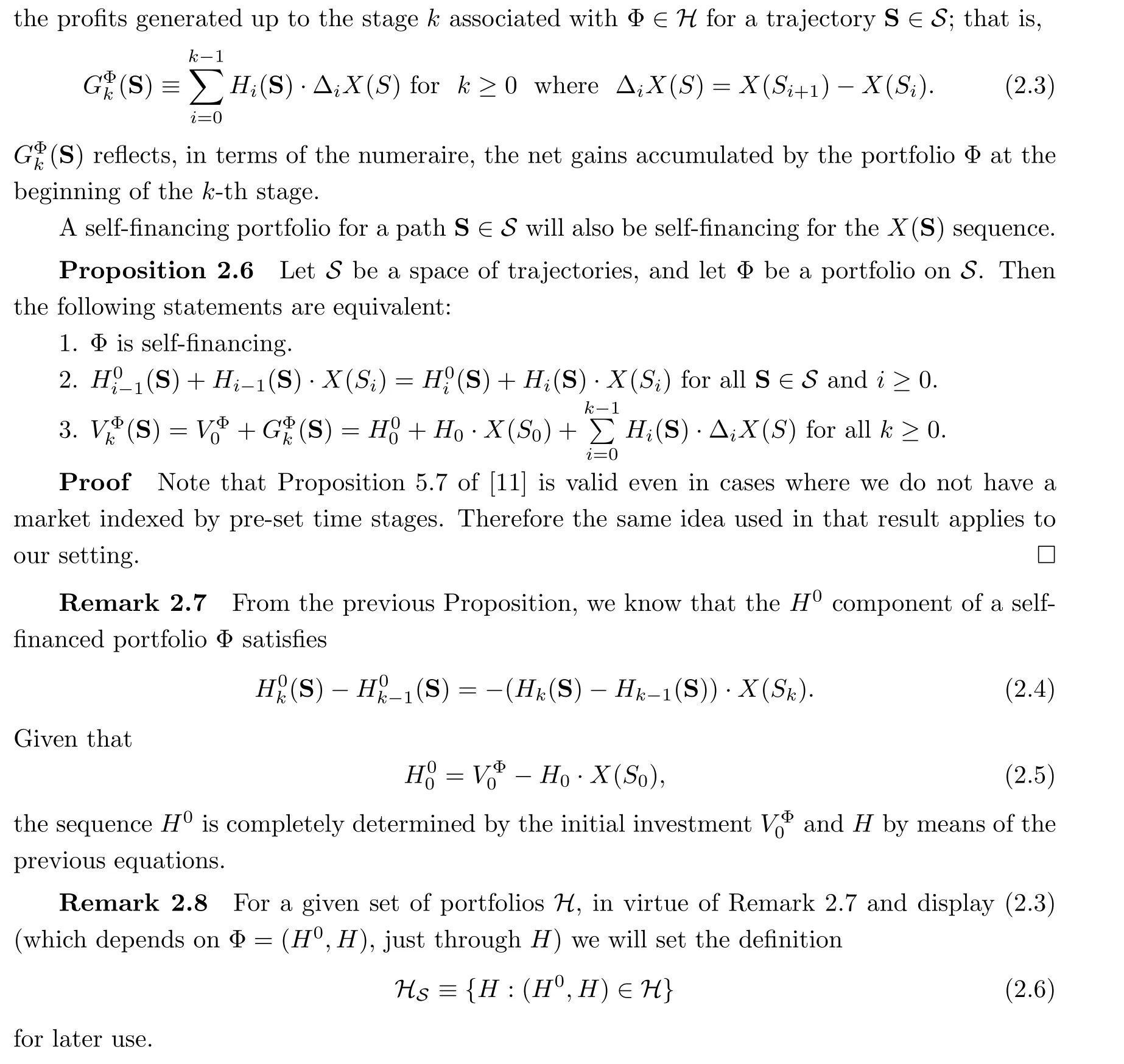
Definition 2.9 (Trajectory market) Given s0∈Rd+1， w0∈Ω0， a trajectory based set S ⊆S∞(s0，w0) and a portfolio set H， we say that M=S×H is a trajectory based market if it satisfies the following properties:

1. For each S ∈S， the coordinate S0i＞0 for all i ≥0.

2. All Φ ∈H are self-financing and Φ=0 belongs to H.

3. For each (S，Φ) ∈M there exists NΦ(S) ∈N such that Φk(S) = ΦNΦ(S) = 0 for all k ≥NΦ(S).

We will say that the market is semi-bounded if， for each Φ ∈H， there is nΦ∈N such that NΦ(S)≤nΦfor all S ∈S and that it is n-bounded， for n ∈N， if NΦ(S)≤M(S)≤n for each pair (S，Φ)∈M. A portfolio set H obeying items (2) and (3) above will be called admissible.

The third property of the previous definition states that the adjustments of the portfolio Φ for a trajectory S will end at， or before， the stage NΦ(S)-1， which means that the portfolio was liquidated on， or before， the period NΦ(S). In this case， the corresponding portfolio will be called liquidated.

The above setting incorporates，as a special case，a discrete time stochastic model. Given a process Y ={Yi=(Y0i ，...，Ydi )}i≥0on a probability space (Ω，P) with filtration F ={Fi}i≥0and F0being trivial， Yki :Ω →R， Yki ∈Fi. We can then define S ={S={(Si≡Yi(ω))}i≥0:for some ω ∈Ω}. One can also define a set of trajectories S by means of a sequence of admissible stopping times τ = {τi}i≥0: S ∈S， so S = {(Si≡Yτi(ω)(ω))}i≥0for some ω ∈Ω.Another way to proceed is to use a given collection of such sequences of stopping times; for the details of this we refer to Section 6 in [9].

3 Arbitrage and 0-Neutrality

A model for common market situations should not allow for investors that are able to generate a profit in a transaction without any risk/possibility of losing money. Such an investment opportunity is called an arbitrage opportunity.

Definition 3.1 (Arbitrage opportunity) Given a trajectory based market M = S ×H，Φ ∈H is an arbitrage opportunity if

· ∀S ∈S， VΦNΦ(S)≥VΦ0 ;

· ∃S*∈S such that VΦNΦ(S*)＞VΦ0 .

We say that M is arbitrage-free if H does not contain arbitrage opportunities.

The particular case S0i=1， for all i， gives X(Si)=(S1i，...，Sdi); i.e. the original currency is the asset S0and is being used as numeraire， and so [S0i] = $/$. Currency， if included as a traded asset and in the presence of a riskless bank account with non-zero interest rates， will lead to an arbitrage as per Definition 3.1. That is， currency， under the mentioned conditions，will be banned as a traded asset whenever we assume a no arbitrage market (as well as a 0-neutral market). Notice the relevant discussion in[19]about arbitrage and non-arbitrage assets，currency being an arbitrage asset (in contrast to an interest bearing money market account).

Our use of an arbitrary value for VΦ0in the definition of an arbitrage opportunity is nonstandard; textbook definitions require that VΦ0≤0 (see [11]). One can see that the existence of an arbitrage as per Definition 3.1 is equivalent to the existence of an arbitrage portfolio ˜Φ with V˜Φ0=0，and so proving the equivalence of our definition and the standard definition. This equivalence allows us also to show that Definition 3.1 is invariant under a change of numeraire and so the latter transformation will be a no arbitrage symmetry according to our definitions;this we show explicitly by a different argument in Corollary 5.7.

The arbitrage-free condition is sufficient for the model to provide fair option prices (a well known result in the classical financial literature.) One can relax the arbitrage free criteria to the requirement that the largest of the minimum possible gains that can be obtained by means of the strategies available in the market is 0. This notion was originally presented in [3] (as equivalent with arbitrage-free) and then formally defined and clarified for the case of a single risky asset in [9] and [6].

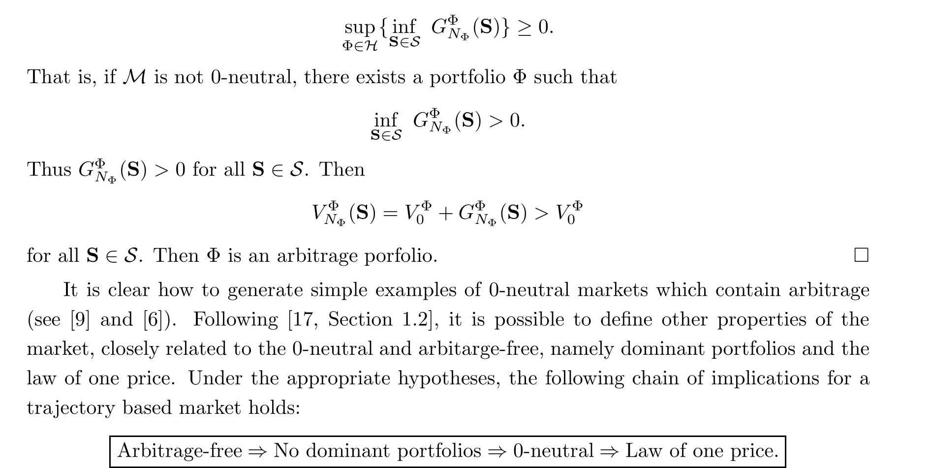
Definition 3.2 (0-neutral market) Let M = S ×H be a trajectory based market. We say that M is 0-neutral if

In[9]it is shown that this property is also sufficient to obtain a pricing interval for financial derivatives. The next proposition shows that 0-neutrality is weaker than arbitrage-free.

Proposition 3.3 Let M = S ×H be an arbitrage-free trajectory based market. Then M is 0-neutral.

Proof We are going to prove the proposition by contraposition. Note that if M=S×H is a trajectory based market 0 ∈H， then it is always true that

At this point，we have introduced enough properties of multidimensional trajectory markets in order to address our goal of characterizing no-arbitrage symmetry transformations.

3.1 Relationships Between Local and Global Properties

From the definitions，it is not clear how to construct arbitrage-free or 0-neutral markets. For the case of semi-bounded markets， one can obtain necessary and sufficient conditions only by involving local properties of the trajectory set，implying trajectorial markets that are arbitragefree (or 0-neutral). Such characterizations play an analogous role to the equivalence of no arbitrage stochastic markets and the possibility to equivalently modify the stochastic process into a martingale process. In fact， in the arbitrage-free case， the local trajectorial conditions correspond to a probability free notion of a martingale sequence (see [10]). We will use these characterizations to pose and answer our opening question on no-arbitrage preserving transformations.

At the k-th stage， the information about the future available to investors is that S is an element of the set

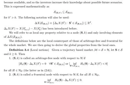
M is called locally arbitrage-free(0-neutral)if each (S，k) is an arbitrage-free(0-neutral) node w.r.t. H. A node that is not arbitrage-free w.r.t. H， will be called an arbitrage node w.r.t. H.

Notice that an arbitrage-free node w.r.t. H is always 0-neutral w.r.t. H. Clearly， there are natural examples of nodes which are 0-neutral w.r.t. H， but no arbitrage-free w.r.t. H (hence these are arbitrage nodes). It is then of interest to indicate that there are results ([9]) that justify option prices obtained for general 0-neutral markets (in particular， these markets may contain 0-neutral nodes which are arbitrage nodes w.r.t. H).

Admittedly， attaching the qualifier“w.r.t. H”to some of the above notions does not play a substantial role in our paper. In fact，Proposition 3.5 below provides sufficient conditions on trajectory nodes that imply that those nodes are arbitrage-free(0-neutral)w.r.t. any(admissible)H.

The conclusions in Proposition 3.5 below are consequences of characterizations given by Propositions 4.2 and 4.4 in Subsection 4.1.

Results and notions from convex analysis that we will rely upon throughout the rest of the paper are detailed in Appendix A.2.

In accordance with these results，we introduce the following notions which will play a crucial role throughout the remainder of the paper:

Definition 3.6 (H-Independent local properties) A node (S，k) is called arbitrage-free if (3.1) is satisfied; it is called 0-neutral if (3.2) is satisfied. We call S locally arbitrage-free(locally 0-neutral) if every node (S，k) is arbitrage-free (0-neutral).

Remark 3.7 The above definitions rely on a numeraire(through the perspective function X). We will show in Section 5 that once the properties hold for one numeraire， they hold for any numeraire.

Therefore， if S is locally arbitrage-free (locally 0-neutral)， then M = S × H is locally arbitrage-free (locally 0-neutral) for any (admissible) H.

Remark 3.8 Condition(3.1)appears in the stochastic literature as equivalent to one step arbitrage-free markets ([4， Lemma 3.42]， [7， Prop 3.3.4]， [11， Cor 1.50]， [13]).

The local notions in Definition 3.6 allow us to ensure global conditions on a trajectory based market. In particular，the results in the rest of this section characterize an arbitrage-free market (0-neutral) by means of arbitrage-free (0-neutral) nodes w.r.t. H.

Theorem 3.9 (No arbitrage: local implies global) If M=S×H is locally arbitrage-free(as per Definition 3.4) and semi-bounded， then M is arbitrage-free (as per Definition 3.1); see Proof of Theorem 3.9 in Appendix A.1.

is self-financing. Also， defining NΞ(S，k)(S′)=k+1 for all S′∈S， it is easy to see that Ξ(S，k)is a portfolio. We will call this type of portfolio a restricted portfolio at the node (S，k).

Proposition 3.10 (No arbitrage: global implies Local) If M = S ×H is arbitrage free and the restricted portfolios belong to H，then S is locally arbitrage-free(as per Definition 3.6).In particular， M is locally arbitrage-free;see Proof of Proposition 3.10 in Appendix A.1.

We now carry out a similar analysis for the notion of 0-neutral. The following Theorem shows that a trajectory based market will be 0-neutral if it is locally 0-neutral:

Theorem 3.11 (0-neutral: local implies global) Let M = S ×H be a semi-bounded trajectory market. If M is locally 0-neutral(as per Definition 3.4)，then M is 0-neutral(as per Definition 3.2); see Proof of Theorem 3.11 in Appendix A.1.

Proposition 3.12 (0-neutral: global implies local) Let M = S × H be a 0-neutral trajectory market such that the restricted portfolios belong to H. Then， any node (S，k) is a 0-neutral node (in particular， (S，k) is 0-neutral with respect to H); see Proof of Proposition 3.12 in Appendix A.1.

4 Geometric Characterizations

We develop geometric characterizations for the local notions introduced in the previous section. Definition 4.1 below is a stronger version of Definition 3.4 that dispenses of the qualifier“w.r.t. H” present in the latter definition.

4.1 Local geometric characterizations

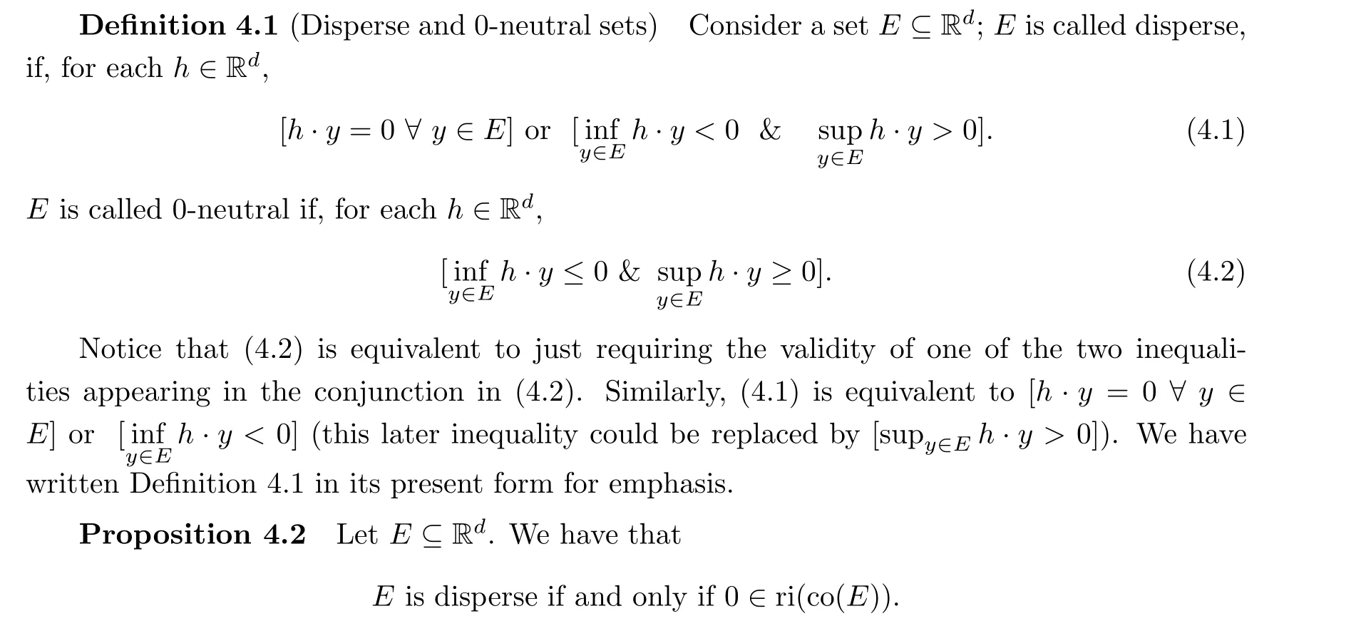
Proof Assume first that E is disperse. In order to proceed to deduce a contradiction，we assume that 0 /∈ri(co(E)); by the separation Theorem A.11， there exists ξ ∈Rdsuch that

· ξ·x ≥0 for all x ∈ri(co(E))， and

· ξ·x*＞0 for some x*∈ri(co(E)).

Then， by means of Proposition A.3， it follows that， for all x ∈ri(co(E))，

4.2 Convexity preserving maps

In order to identify transformations that preserve no-arbitrage(0-neutrality)，and in view of Proposition 4.2(Proposition 4.4)and Lemma 4.5，we first look for transformations F :Rd→Rd′preserving relative interiors or closures of convex sets in Rd.

The notions introduced below are expanded in Appendix A.2， where we also provide due references and introduce related definitions and further results.

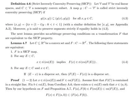
Now， since co(F(E)) is a segment， because it is contained in a straight line， it follows that if b′∈(F(x)，F(b))， or F(b)∈(F(x)，b′)， then F(x)∈(F(a)，b′)⊂co(F(E)). On the other hand，F(x)∈(F(b)，b′)⊂co(F(E)). Thus， in any case， by Corollary A.6， F(x)∈ri(co(F(E))).

If F(C) is not contained in a straight line， by Theorem A.10，F preserves segments strictly and co(F(E))=F(co(E))， so b′=F(b) with b ∈co(E).

As before， there exists a ∈co(E) such that x ∈(a，b). Then F(a) ∈co(F(E)) and F(x)∈F((a，b))=(F(a)，F(b))， which also leads to F(x)∈ri(co(F(E))).

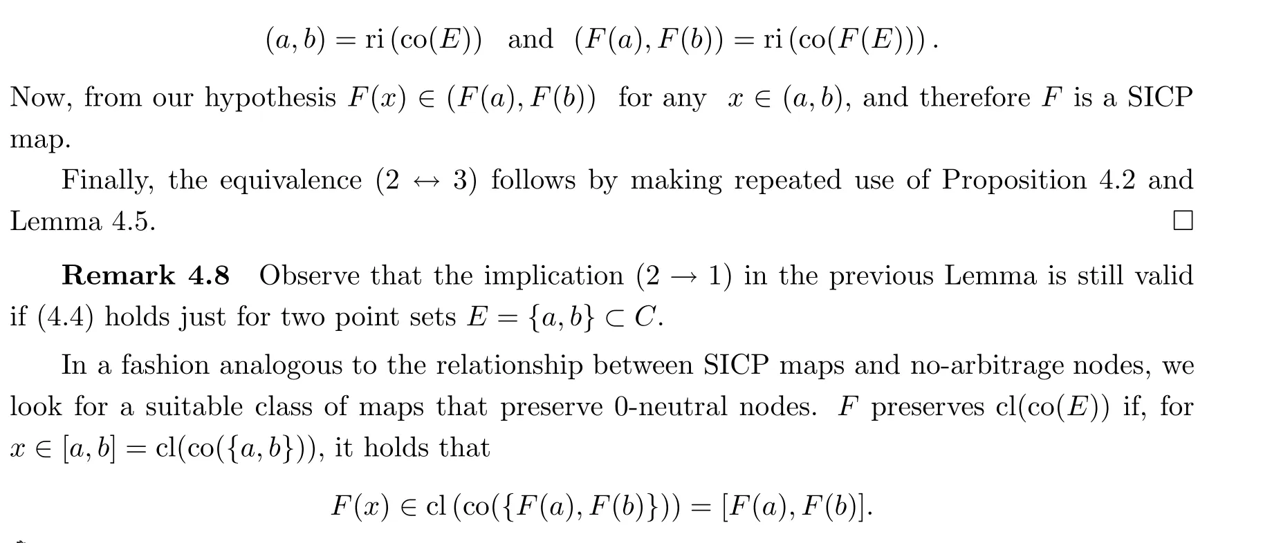
(2 →1) Considering the case E ={a，b}，

4.3 Induced transformations

As indicated in Section 2.1， we have taken a standard view in which the original sequence Siis given in a currency numeraire and then the sequence X(Si)is given in another(arbitrary)numeraire. Since we look for transformations between trajectories of financial markets that preserve their local properties， we will be dealing with two associated functions， f and F， the former acting on Siand the latter on X(Si). Thus，we will have Rd+1f-→Rd′+1and RdF-→Rd′.One could proceed differently and develop an approach which abstracts away this multiplicity;nonetheless，we have decided to proceed the way we do，as in practice that is how data is usually presented. This decision makes our results more readily applicable， albeit at the price of some complications.

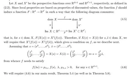
Lemma 4.7 will be used in Corollary 5.6 to establish that the SICP property for the induced map F is necessary and sufficient for f to preserve the no-arbitrage property of any given node in any locally arbitrage-free trajectory set. Lemma 4.11 item 1， below， provides sufficient conditions on f to establish the SICP property of F; on the other hand， Example 4.12 shows that the assumptions on f， while being sufficient， are not necessary.

Lemma 4.11 Let f :dom X →dom X′be a function satisfying (4.6). Then there exists a unique map F :Im X →Im X′which makes commutative the diagram (4.5). Moreover，

1. if f is (strict) inversely convexity preserving， then F is (strict) inversely convexity preserving;

2. F is continuous if and only if f is continuous.

Proof For all x ∈Im X， there exists s ∈dom X such that X(s) = x. The only way to define F is then F(x)=X′(f(s)) for all x ∈Rd， and it is well-defined by condition (4.6).

Let us see that F is a SICP map if f is assumed to satisfy that property. Fix ˆx，˜x ∈Im X and let x ∈Im X such that x=αˆx+(1-α)˜x with 0 ＜α ＜1. Then，there exists ˆs，˜s ∈dom X such that X(ˆs) = ˆx and X(˜s) = ˜x. Moreover， since X is a strict segment preserving map(Theorem A.9)， there exists β ∈(0，1) such that

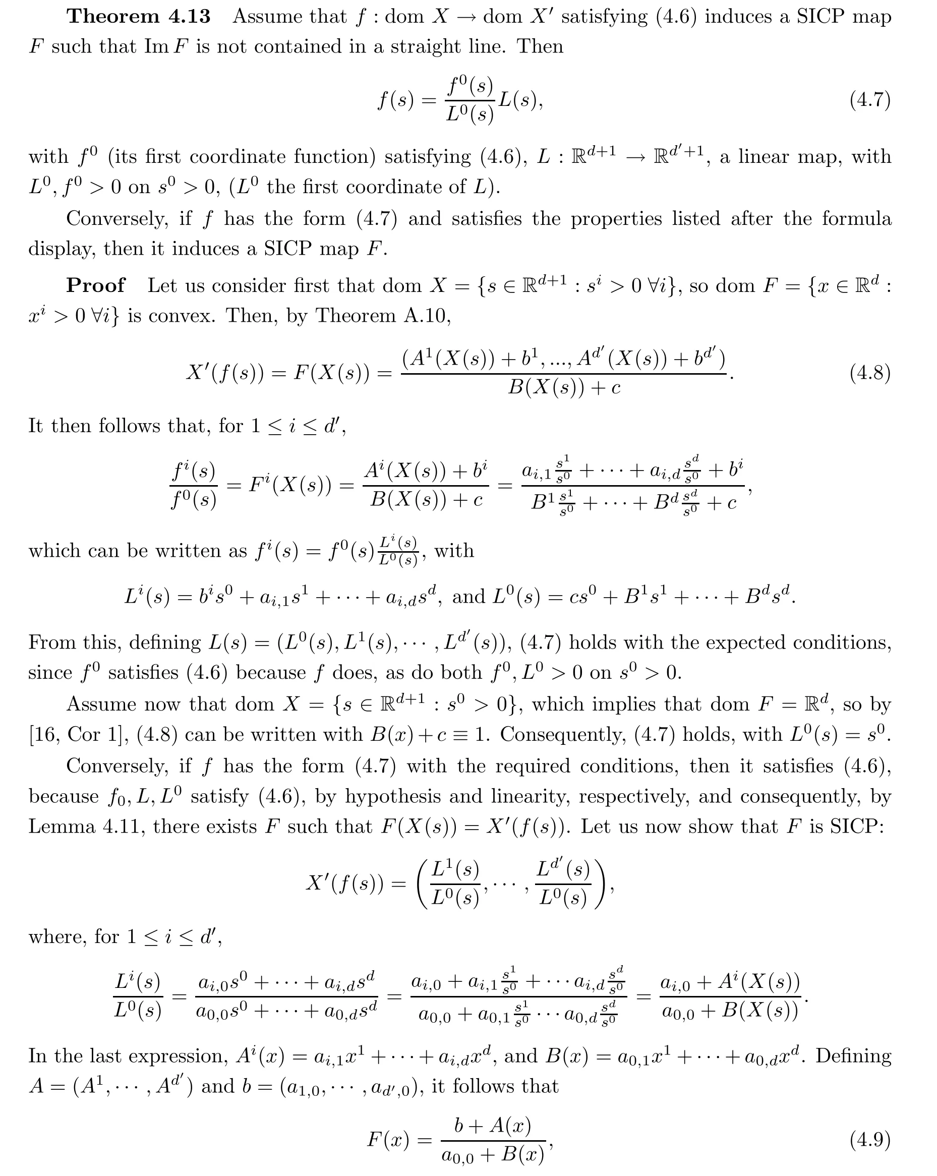
which is SICP， by Theorem A.9. □

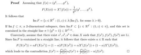
Lemma 4.14 Assume that f :dom X →dom X′is a function satisfying (4.6) and that F is the induced function as in Lemma 4.11. Then， Im F is contained in a straight line if and only if Im f is contained in a 2-dimensional subspace.

5 No Arbitrage Invariance

This section studies a class of transformations that do not change a given node’s local properties of being arbitrage-free (this latter notion as per Definition 3.6). We also provide an explicit characterization for such symmetry transformations; this is achieved under a general and weak condition restricting their ranges.

As a special case，we will prove that the no-arbitrage property is unchanged under a change of numeraire. We also describe similar results that apply for the property of 0-neutrality，and therefore need to also pursue some developments that apply to this concept as well. In general， the class of transformations studied should represent symmetries obeyed by any type of functional relationship among assets’ prices resulting from no arbitrage considerations. In particular， if prices S satisfy a h(S) = 0 relation， one then expects h(S′) = 0 where S and S′are related by a no-arbitrage symmetry as per Definition 5.1 below. This fact is illustrated with an example in Section 6.

Definition 5.1 (No-Arbitrage Symmetry (NAS) Transformation) A trajectory transformation f， as introduced above， which leaves invariant the arbitrage-free property (0-neutral property)， as per Definition 3.6， of any locally arbitrage-free (locally 0-neutral) trajectory set S with d+1 assets， will be called a no-arbitrage symmetry (0-neutral symmetry).

More specifically， f :Rd+1→Rd′+1， is a NAS if and only if

and this holds for any possible trajectory set S that is locally arbitrage-free (0-neutral).

Therefore， if the node (S，k) is arbitrage-free， so too will be (S′，k) if f is a no-arbitrage symmetry (similarly for a 0-neutral symmetry)， and this is required to hold for any trajectory set S that is locally arbitrage-free. This remark also shows that the composition of no-arbitrage symmetries (0-neutral symmetries) is a no-arbitrage symmetry (0-neutral symmetry). We may refer to either type of symmetry as NAS (No-Arbitrage Symmetries) when there is no need to be specific.

Remark 5.2 The above notions depend on a choice of numeraire through Definition 3.6，but we will prove in Corollary 5.7 that a symmetry transformation remains as such under a numeraire change. Of course， the interest is in general symmetry transformations f : Rd+1→Rd′+1that behave so for any possible node in any possible trajectory set (with corresponding dimension d and satisfying the arbitrage-free/0-neutral property)， as we have required in our definition.

The next proposition (which follows from Proposition 3.5 in Section 3.1 and Lemma 4.5 in Section 4.2) shows that local conditions can be rewritten in terms of the set Σk(S).

Proposition 5.3 Given a trajectory based set S，S={(Si，Wi，m)}i≥0∈S and an integer k ≥0，

1. the node (S，k) is arbitrage-free if and only if X(Sk)∈ri(co(X(Σk(S))));

2. the node (S，k) is 0-neutral if and only if X(Sk)∈cl(co(X(Σk(S)))).

Theorem 5.4 (Arbitrage-Free Invariance) Assume f : dom X →dom X′to be a map satisfying(4.6)，and that the function F，induced by Lemma 4.11，is SICP.Given a trajectory set S，let S ∈S and k ≥0. If(S，k)is an arbitrage-free node，then(S′，k)，where S′i=f(Si) i ≥0，is an arbitrage-free node in the transformed trajectory set S′; that is，

Proof We know from Lemma 4.11 that there exists F : dom X →dom X′given by F(x)=X′(f(s))，where s ∈dom X such that X(s)=x. Thus，since，by hypothesis，it is a SICP map， from Proposition 5.3 and Lemma 4.7， it follows that F(X(Sk))∈ri(co(F[X(Σk(S))])). □

Remark 5.5 By Lemma 4.11 item 1， if f satisfies (4.6) and it is SICP， then the induced F satisfies the hypothesis of Theorem 5.4. Also notice that if ImF contains a nondegenerate triangle， by Theorem 4.13， f is of the form given by (4.7).

Corollary 5.6 (Explicit Characterization) Assume that f : dom X →dom X′satisfies(4.6). We then have the following:

1. If f is a no-arbitrage symmetry (as per Definition 5.1)， then F (as appearing in Lemma 4.11)is SICP. Moreover，if Imf is not contained in a 2-dimensional subspace，then f is characterized by expression (4.7).

2. Conversely， if f has the form (4.7)， then it is a no-arbitrage symmetry.

Proof We recall that (4.6) assures us of the existence of the induced function F as in Lemma 4.11. Assuming that f is a no-arbitrage symmetry for trajectory sets with d + 1 assets， then， for any node (S，k) from a locally arbitrage-free trajectory set S， by Proposition 5.3， F verifies that F(X(Sk)) ∈ri(co(F[X(Σk(S))])). Since for any a，b ∈Rdand x ∈(a，b) = ri(co({a，b}))， there exists a binary trajectory set with a node (S，k) such that ri(co(X(Σk(S))))=ri(co({a，b}))and X(Sk)=x， it then follows from Lemma 4.7 (see Remark 4.8) that F is SICP. Moreover， if Im f is not contained in a 2-dimensional subspace， Lemma 4.14 implies that Im F is not contained in a straight line. Finally by Theorem 4.13，f takes the form (4.7). This proves 1.

For the converse， if f has the form (4.7)， the converse of Theorem 4.13 implies that the induced function F is SICP.Thus by Lemma 4.7 and Theorem 5.4，f is a no-arbitrage symmetry.

□

Observe that the composition of no-arbitrage symmetries of the form (4.7) is again of this form.

A transformation of interest in financial terms is the one that changes the market model’s numeraire. Let us take S with S0k，S1k＞0， for all k ≥0 and all S ∈S. For the purposes of the next proposition， let S′be defined by S′∈S′if and only if S′k=f(Sk) for some S ∈S， where f(s0，s1，s2，...，sd)≡(s1，s0，s2，...，sd).

Corollary 5.7 (Change of Numeraire is a NAS) Consider S to be a trajectory set such that S0k，S1k＞0 for all k ≥0 and all S ∈S， and let S′and f be as introduced above. Then， if S is locally arbitrage-free， it follows that S′is locally arbitrage-free as well.

Proof Since f is a linear map， it follows from Theorem A.9 in Appendix A.2 that it is a strict segment preserving map (in particular it is a SICP map). From Remark 5.5 we see that Theorem 5.4 applies to our particular f. Therefore， f is a NAS， and so (5.1) implies that S′is locally arbitrage-free. □

Our next goal is to find market transformations f that preserve 0-neutral nodes (i.e. 0-neutral symmetries). From Lemma 4.9 we know that the induced transformation F needs to be continuous and inversely convexity preserving in order to preserve the closure of convex sets. The following Theorem shows that these conditions are sufficient to obtain a 0-neutral symmetry， as per Definition 5.1:

Theorem 5.8 (0-Neutral Invariance) Let f : dom X →dom X′be a continuous map satisfying (4.6) and the function F， induced by Lemma 4.11， is inversely convexity preserving.Given a trajectory set S， let S ∈S and k ≥0. If (S，k) is a 0-neutral node， then (S′，k)， where S′i=f(Si) i ≥0 is a 0-neutral node in the transformed trajectory set S′， i.e.，

so f is a 0-neutral symmetry.

Proof We know from Lemma 4.11 in Section 4.2 that there exists a continuous map F :Rd→Rd′， given by F(x)=X′(f(s))， where s ∈dom X such that X(s)=x. Moreover，by hypothesis， this map is inversely convexity preserving.

Thus， since， by hypothesis， X(Sk)∈cl(co(X(Σk(S))))， from Lemma 4.9 in Section 4.2， it follows that X′(f(Sk))∈cl(co(X′(f(Σk(S))))). □

By the converse of Theorem 4.13，if f is given as in the expression(4.7)，with the prescribed conditions， then the induced function F has the expression(4.9). Therefore，it is also inversely convexity preserving and continuous by Theorem A.9，so f preserves 0-neutral nodes and hence，it is a 0-neutral symmetry.

In the 0-neutral market definition， the selection of an explicit numeraire is required. The proof of the next result is analogous to Corollary 5.7， and so it is omitted.

Corollary 5.9 (Change of Numeraire is a 0-Neutral Symmetry) Consider S to be a trajectory set such that S0k，S1k＞0 for all k ≥0 and all S ∈S， and let S′and f be as in Corollary 5.7. Then， if S is locally 0-neutral， it follows that S′is locally 0-neutral as well.

6 Example

We will provide a slightly non-traditional development on the call-put parity relationship.This is a simple relation among prices of certain assets;it is derived in many textbooks and can be obtained through a no-arbitrage based proof. We will derive it under the weaker hypothesis of 0-neutrality and relate the relationship to NAS (No-Arbitrage Symmetries). Our main point of revisiting the call-put parity is that it will allow us to provide an explicit example of NAS(besides a change of numeraire) as well as to illustrate their meaning in this context.

6.1 Call-Put Parity Under 0-Neutrality

That is， under the said conditions， no-arbitrage constrains the evolution of the four assets according to (6.1).

We will add details on dimensions that are neglected in the above formulation; dispensing with units/dimensions is standard in the literature but making them explicit is relevant to our philosophy as a change of units should be a NAS (but we do not explore this view in the paper). We will insert appropriate dimensions/units whenever relevant but switch(or alternate)to suppressing units (as usual) whenever the relevant dimensions have been made clear. We write Z =(Z)[Z] where (Z)is the (dimensionless)numerical value and[Z]are the dimensional units of the variable Z.

6.2 Proof of call-put parity

6.3 An example of a NAS

6.4 Call-put parity under a no-arbitrage symmetry

Let us now see the effect on the call-put parity relation after applying a no-arbitrage symmetry. Towards this end， consider f to be a no-arbitrage symmetry satisfying (4.6) and such that Im f is not contained in a 2-dimensional subspace. From Corollary 5.6， we have that

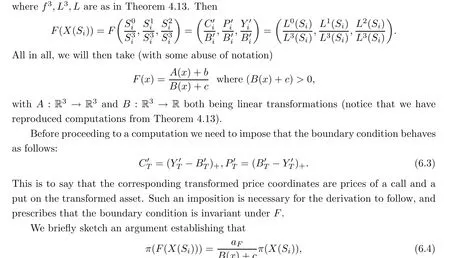
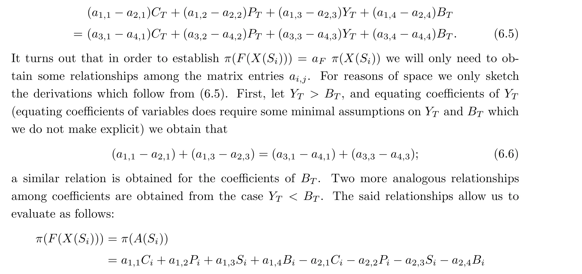
where aF≡(a1，1-a2，1-a3，1-a4，1) and aj，kare the matrix coordinates of a matrix representation of A. The relationship (6.4) makes it immediately apparent that π(X(Si)) = 0 implies π(F(X(Si)))=0， and hence reflects the notion of symmetry embodied by F. The implication π(X(Si))=0 =⇒π(F(X(Si)))=0 is known to us without recourse to(6.4);this is so because f is a no-arbitrage symmetry and so is a 0-neutral symmetry， and given that S is assumed to be 0-neutral， so then will S′be (this trajectory set is obtained from S by acting with f on the trajectories S ∈S).

Given that π is linear， it is enough to consider the case F(x) = A(x) and to establish the existence of aFsuch that π(F(X(Si)))=aFπ(X(Si)).

To start， substracting the two equations in (6.3) we obtain that

7 Conclusion

The paper poses and solves the following basic question: what transformations， acting on financial events， leave the no-arbitrage property invariant? Such transformations are called no-arbitrage symmetries (NAS) and are interpreted as mapping financial events to financial events. We make use of results from convex analysis and a general non-probabilistic framework to characterize and provide explicit expressions for the NAS.We take advantage of a formulation of arbitrage free markets(as per Section 4)in terms of geometric assumptions of the trajectories in discrete time. The problem formulation naturally provides the characterization， in a local sense， of no-arbitrage preserving transformations.

The transformed variables， i.e. the output values of NAS， do require an interpretation，as the original setting is abstract and general. For instance， in Section 6 we have to impose that boundary conditions should also be invariant under NAS， and in so doing we required that two of the transformed variables acted as call and put options on the two remaining transformed variables. From such a general point of view， we think that the results of applying a NAS to financial events are admissible prices for financial events， but the latter will require an interpretation that will depend on the context and the specific NAS under consideration.

Appendix

A.1 Results and proofs from section 3

The following simple characterization of 0-neutral markets is used in one of our results:

Proposition A.1 A trajectory based market M= S×H is 0-neutral if and only if， for each Φ ∈H and ∈＞0， there exist S∈∈S such that

for any ∈＞0. Thus we have proved the necessary condition.

For the sufficient condition， fix ∈＞0. Then，by hypothesis，for each Φ ∈H， there is S∈∈S such that

therefore Φ is not an arbitrage opportunity.

We may then assume that there exists a trajectory S(0)∈S and an integer k ≥0 such that， at the node (S(0)，k)， Hk(S(0))·ΔkX(S)/=0 for some S ∈S(S(0)，k).

Then，by Definition 3.4，1.，it is possible to choose k1，0 ≤k1≤k as the smallest integer such that， for 0 ≤j ＜k1， Hj(S)·ΔjX(S)=0 for all S ∈S(S(0)，j)， and there exists S(1)∈(S(0)，k1)such that

To begin， let us remember the notion of relative interior， which will be very important in the characterizations of local properties.

Definition A.2 (Relative interior) Let E ⊂Rdbe a convex set. The relative interior of E， that we will denote by ri(E)， is the interior of the set relative to its affine hull， that is，

Proposition A.7 Letting g :Rd→Rd′，

1. g preserves convexity if and only if [g(x)，g(y)]⊆g([x，y]) for all x，y ∈Rd;

2. g is inversely convexity preserving if and only if g([x，y])⊆[g(x)，g(y)] for all x，y ∈Rd.

Note that it follows from the previous Proposition that a convexity preserving function which is， at the same time， inversely convexity preserving， satisfies [g(x)，g(y)] = g([x，y]) for all x，y ∈Rd. This motivates the following definition:

Definition A.8(Segment preserving) We say that a map g :Rd→Rd′preserves segments if [g(x)，g(y)] = g([x，y]) for all x，y ∈Rd. If (g(x)，g(y)) = g((x，y)) for all x，y ∈Rd， we say that g preserves segments strictly.

Then， g preserves segments if and only if g preserves convexity and preserves convexity inversely. Clearly， if g preserves segments strictly， then it preserves segments; the converse，however，may not be valid.

The obvious candidates for being functions that preserve segments strictly are the affine functions. Recall that a function g :Rd→Rd′is affine if it is the sum of a linear function plus a constant， that is: g(x) = Ax+b， where A ∈Rd×d′and b ∈Rd′. There is a larger class of functions which also preserve segments strictly.

Theorem A.9 ([16， Theorem 1]) Let A: Rd→Rd′and B : Rd→R be linear functions and b ∈Rd′and c ∈R. Let D ={x ∈Rd:B(x)+c ＞0}. Then: g :D →Rd′， given by