Causality fields in nonlinear causal effect analysis＊

Aiguo WANG，Li LIU，Jiaoyun YANG，Lian LI

1 School of Electronic In formation Engineering，Foshan University，Foshan 528225，China

2School of Big Data&Software Engineering，Chongqing University，Chongqing 400044，China

3School of Computer Science and Information Engineering，Hefei University of Technology，Hefei 230009，China

E-mail:wangaiguo2546@163.com;dcsliuli@cqu.edu.cn;jiaoyun@hfut.edu.cn;llian@hfut.edu.cn

Compared with linear causality，nonlinear cau‐sality has more complex characteristics and content.In this paper，we discuss certain issues related to nonlinear causality with an emphasis on the concept of causality field.Based on widely used computation models and methods，we present some viewpoints and opinions on the analysis and computation of non‐linear causality and the identification problem of cau‐sality fields.We also reveal the importance and prac‐tical significance of nonlinear causality in handling complex causal inference problems via several specific examples.

1 Introduction

According to the three-level causal hierarchy proposed by Judea Pearl，having the knowledge of causality rather than correlation endows us with the ability to better answer the critical questions related not only to association，but also intervention and counter‐factuals(Pearl，2019).In principle，causality studies the cause–effect relationship，and thus helps reveal the data generation procedure.However，statistical corre‐lation does not necessarily indicate causation.For example，a positive correlation between yellow fingers and cough is falsely generated by smoking.In this case，smoking is the common cause(i.e.，confounder)of both yellow fingers and cough，and we cannot say that yellow fingers causally lead to cough.The Simpson paradox，in which uncontrolled and even unobserved variables could reverse or eliminate an association be‐tween two variables，is a typical phenomenon in prob‐ability and statistics.For example，the COVID-19 case fatality rate in Italy is higher than that in China overall，but for age groups，the case fatality rates in Italy are lower than those in China(von Kügelgen et al.，2021).One strategy to treat this phenomenon is to use causality.In addition，causal inference contributes to the devel‐opment of machine learning in better solving open problems(e.g.，explainability，robustness，adaptability，and transfer learning)and further paves the way for next-generation artificial intelligence with the abili‐ties such as reflection and reusable mechanisms(Yue et al.，2020;Schölkopf et al.，2021).Therefore，un‐derstanding and analyzing cause–effect relationships is of great value and of primary interest in a variety of fields，e.g.，economics，education，genomics，epide‐miology，and medical science(Stavroglou et al.，2019).

Although significant progress has been achieved in causal inference，to our knowledge，most of exist‐ing studies deal with linear causal inference，while little attention has been devoted to nonlinear causal inference(Guo et al.，2021;Yao et al.，2021).To this end，we present some viewpoints and opinions on nonlinear causal inference，including its definition，characteristics，and its differences to linear causal inference，especially the causality field problem.

2 Causality fields

We first present related notations before illus‐trating the nonlinear causal effect.Suppose thatDis a set of data points andu∈Dis defined by

wherexi(i=1，2，…，n)denotes theithvariable(feature)andaiindicates its corresponding value.Specifically，aican be binary，multi-valued，or continuous，andu=(a1，a2，…，an)when there is no ambiguity.Although the binary case ofaiis the simplest and perhaps the most commonly used one in practice，we are often required to handle multi-valued，discrete，and even continuous values in the nonlinear causality problem.

Given the cause variableX，effect variableY，variableZthat influencesXandY(often called the covariable in the potential outcome framework，or the backdoor variable in the causal structural model)，and exogenous variableU，we can obtain Eq.(2)，known as the structural causal equation(SCE)，via the datafitting or regression methods(Rubin，2005;Pearl，2009).

The average causal effect(ACE)for discrete variables is denoted by Eq.(3):ACE(X→Y)

It is known that ACE(X→Y)indicates the causal effect ofXonYby measuring the change inYfor a one-unit change inX.For a continuous case，it is expressed as ACE(X→Y)|X=x

which essentially estimates the ACE atX=x.

Obviously，iff(X，Z，U)=aX+b Z+c U，which is a linear equation，Eqs.(3)and(4)would return ACE(X→Y)=a;that is，the causal effect equals the coefficientaofXirrespective of the values ofZandU，which is a characteristic of linear causality.However，it raises complex issues for the nonlinear case.Then，we present the definitions and characteristics related to nonlinear causal analysis.

Definition 1(Nonlinear causality) If the functional relationshipf(X，Z，U)is nonlinear，the causal relation betweenXandYis called nonlinear causality.

For nonlinear causality，the causal effect ofXonYdepends not only onXbut also onZandU，and different values ofX，Z，andUlead to different ACEs.Consequently，this makes nonlinear causality different from linear causality to a large extent and complicates the nonlinear causal effect.Specifically，we can divide the nonlinear causal effect into strong nonlinear and quasi-linear types.

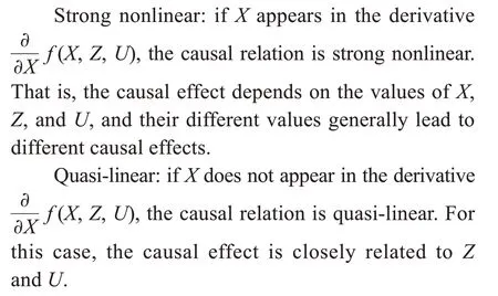
This indicates that the expectation of ACE(X→Y)in quasi-linear causality may vary only with the values ofZandU，and that the expectation of ACE(X→Y)in strong nonlinear causality depends also on the value ofXbesidesZandU.For the purpose of explanation，Table 1 gives an illustrative example，whereX=1 indicates the treatment group(drug taker)，X=0 is the control group(drug nontaker)，Yhas three outcomes，including recover(Y=1)，worsen(Y=-1)，and unchanged(Y=0)，andZ={1，0}denotes daytime and night respec‐tively.Zinfluences both treatmentXand effectY.Suppose that the results of drug test effectiveness are as shown in Table 1.The SCE is

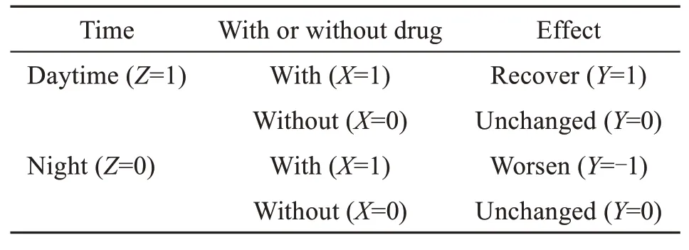
Table 1 The effect of a drug considering the time

This case is obviously quasi-linear.According to Eq.(3)，we can obtain

However，we have ACE∣Z=1=E(Y∣do(X=1)，Z=1)-E(Y∣do(X=0)，Z=1)=1 forZ=1，and ACE∣Z=0=E(Y∣do(X=1)，Z=0)-E(Y∣do(X=0)，Z=0)=-1 forZ=0.Obviously，ACEs are different for differentZvalues.That is，the causal effect ofXonYis fluctuant and related toZ，where there is a positive effect during daytime(i.e.，taking the drug helps recovery)and a negative effect at night(i.e.，the condition worsens upon taking the drug).Thus，if we conclude from ACE=0 that there is no causal effect ofXonY，it does not conform to the facts or our common sense.This indicates that，in con‐trast to the linear causal effect，the expectation ofZprobably counteracts the positive and negative effects in quasi-linear causality，and subsequently yields fluc‐tuating interdependencies ofXonYexisting in the nonlinear causal effect.This example prompts us to consider the problem of nonlinearity in causality anal‐ysis.Obviously，one naive solution is to calculate the causal effects with respect to each value ofZ.

To better illustrate the characteristics of non‐linear causality，we introduce the concept of causality field.

Definition 2(Causality field) This consists of the following three types of causal effect ofXonY:

Positive causality:Xcauses a homodromous change inY;

Negative causality:Xcauses an antagonistic change inY;

Null causality:Xcauses no change inY.

The three fields are noted as

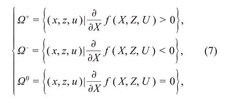
called the causality fields ofXonY.

For linear causality，the causal effect is constant and is independent ofX，Z，andU.However，the causal effect is fluctuant for nonlinear causality，which requires us to identify different causality fields for solving a specific problem.

Next，we study a complex example:the typical competitive–symbiotic relationship between two bio‐logical populations，rabbits and foxes.Such a relation‐ship is given by the following differential equation，the so called Lotka–Volterra equation(Takeuchi et al.，2006;Sugihara et al.，2012):

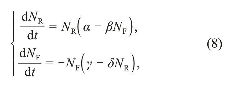
whereNRdenotes the number of rabbits，NFdenotes the number of foxes，tdenotes time，dNR/dtand dNF/dtrepresent the instantaneous growth rates of rabbits and foxes respectively，andα，β，γ，andδare positive real parameters.

Fig.1 presents the illustration plot，where the arrows denote the population trends between rabbits and foxes.We can observe that rabbits and foxes have competitive and symbiotic relationships.For example，under different conditions，an increase in the population size of rabbits can lead to the increase in the population size of foxes(i.e.，areaA，ecological mutualism model)，the decrease in the population size of foxes(i.e.，areaB，ecological competition model)，or the decrease in both the rabbit and the fox population(i.e.，areaC，ecological total-loss model).Obviously，the population of rabbits affects that of foxes under a certain causality existing between them;however，this causality fluctuates between positive and negative values，and has different patterns in different fields.Particularly，null causality exists at the boundary between the positive and negative regions，although its probability measure may be zero.Therefore，the use of ACE probably distorts the true causality and fails to reflect the quantitative relationships between two species.In this situation，the causality field is an important concept to study these relations.

Fig.1 Relationship between two biological populations，rabbits and foxes

3 Computation for nonlinear causal relation

In this section，we discuss how to estimate non‐linear causality and focus on how to analyze the causality field.First，we introduce the following three assumptions to enable causal effect estimation，which play a crucial role in the calculation and analysis of causal effects(Rubin，2005):

Assumption 1(Stable unit treatment value assump‐tion，SUTVA) SUTVA states that the potential out‐come of a unit(or individual)iis independent of the treatment applied to other units，and that two units having the same treatment value would receive the same treatment.SUTVA basically involves no inter‐ference and the well-defined treatment levels.It indi‐cates that there is no difference between the assign‐ments of the treatment group and control group;that is，the experimental results would not change no matter the units are assigned to the treatment or control group.SUTVA is essentially equivalent to the independent causal mechanism(ICM)principle，stating that the causal generative process of variables is composed of autonomous modules that do not inform or influence each other.

Assumption 2(Ignorability) The potential outcomeZis independent of the treatment assignmentXcondi‐tioned on the covariableZ，i.e.，(Y X=1，Y X=0)⊥X|Z，whereY X=x=E Z(Y X=x(z)).This is also called the unconfounder assumption，since it posits the nonexistence of unobserved confounders.However，the means to verify this is a nontrivial task.This assump‐tion enables us to calculate the potential outcome:

which transforms the counterfactual problem into the statistical analysis of observational data.Judea Pearl has proven that ignorability is equivalent to the back‐door criterion(Yao et al.，2021).

Assumption 3(Positivity) This means the choos‐ability treatment assignment，i.e.，P(X=x|Z=z)＞0，∀x，z.This assumption makes the potential outcomes mean‐ingful;otherwise，it is pointless to discuss and calcu‐lateP(Y|X=0，Z)if there are no data points in any case withX=0 conditioned onZ，i.e.，P(X=0|z)=0.

Furthermore，we often call ignorability and posi‐tivity together as strong ignorability.With the above assumptions，we can calculate the ACE.The poten‐tial outcome framework is commonly used to infer the causal effect with regard to the treatment–outcome pair(X，Y|Z)，whereYis the outcome of treatmentXapplied to a population，andZindicates the covari‐able.Then，we define the treatment effect as the differ‐ence between the outcomes of different treatments.Specifically，we useto denote the potential outcome withX=xconditioned onZ=zand define thez-specific causal effect(SCEz)as

whereX=0(X=1)corresponds to the control(treatment)trial.We can also define the ACE over a population:

whereEZis the expectation with respect toZ.Thus，ACE equals the expectation of SCEzassociated withZ.Note thatZshould be the set of backdoor variables.Eq.(11)also embodies the causal effect Eq.(12)pro‐posed by Judea Pearl，such as

WhenX，Z，andYall take binary values，there is no difference between linear and nonlinear causality.However，when they are multi-valued，ACE and SCE probably change following the values ofZ，X，or bothZandX.Specifically，it is more challenging to handle continuous cases.According to the above discussion，ifXis multi-valued，

whereY X=xis the observational outcome of the pres‐ent treatmentX=x，andY X=x′indicates the counterfac‐tual outcome of the imagined treatmentX=x′.The ACE can then be explained as the difference between takingX=xandX=x′.IfX，Z，andYare continuous variables，we obtain the so-called SCE，as show in Eq.(4).

We can observe that ACE depends on the values ofX，Z，andU，which leads to the problem of causality field.In this situation，ACE=0 does not mean that there is no causal effect ofXonY，since their causal effects vary with different causality fields and the ACE could be zero.

However，there are cases where the assumptions do not hold.For example，the interdependency among individuals is clear and unavoidable in the situation of rumor dissemination in social networks，often char‐acterized by the fact that a rumor believed by more people usually generates more people that believe it，which violates the STUVAassumption.

The most popular modeling paradigms might be the causal graphical model and the causal equation model.Machine learning can be seen as a special case of the causal equation model，which is currently popular among researchers.If the graph or the causal equation is given，we can perform a Markov(causal)factorization of the joint distribution(or the term dis‐entangle in machine learning)(Schölkopf et al.，2021):

where PAirepresents the parents of the node(vari‐able)Xi.To learn the causal relations，current approaches typically fall into two categories:constraint-based approaches that use conditional independence tests to determine direct causal relations between observed variables，and score-based approaches that quantita‐tively score possible explanations of the causal rela‐tions(Spirtes and Zhang，2016).Unfortunately，check‐ing the Markov factorization consistency of the rela‐tions from observations and evaluating all possible structures become infeasible with the growth of the modeling size，especially in the case of high-dimensional datasets.This is mainly because it is hard to deter‐mine the directionality between two variables that are statistically dependent and can generate mutual infor‐mation.Most importantly，some datasets are often finite and not causally sufficient(i.e.，unobserved com‐mon causes exist to confound two observed variables).

Compared to the graphical model that describes the observational distribution，SCE is more intuitive for machine learning researchers who are more accus‐tomed to thinking while considering estimating func‐tions rather than probability distributions(Pearl，2019).

wherefidenotes a function andUirepresents an exog‐enous variable.To satisfy causal sufficiency，it is required thatU1，U2，…，Unbe independent according to the common cause principle.Given a set of vari‐ablesX i(i=1，2，…，n)，ifi＜j，without loss of gener‐ality，X j∉PAi，which meansXjwill not be on the right side of the equation ofXi.IfZis the covariable，and the cause variableXand effect variableYare determined，thenXandZmust be the ancestor nodes ofY.Accordingly，we can deriveY=f(X，Z，U)by combini ng t he associated equations and solve i t by applying machine learning models or fitting a model to the raw data.However，we need to know the parent nodes ofXandYto obtain the fitting equa‐tion.We should selectZandUthat influenceXandYbut exclude the variables that are influenced byXorYaccording to the associations in the dataset.This is the key step to derive the fitting equations.Although there are methods currently available，their performance is still unsatisfactory.Typically，for machine learning methods，assumptions on function classes should be given due to the arbitrarily slow convergence.An open research question in the frontier of machine learning is how to derive a model of non‐linear causal relations for a large number of variables，under which the causal inference framework can best exploit the power of machine learning technology.Moreover，additional challenges exist in the era of big data in learning causal relations from high-dimensional data and large-scale mixed data.Recently，a series of causal inference algorithms have been proposed to handle these challenges by employing advanced ma‐chine learning technologies，such as deep learning networks，to identify nonlinear relations.Score-based methods use a scoring function to measure the quality of fitting a causal graph to the data，and a lower score indicates the existence of incorrect conditional inde‐pendence.These methods consist of two components:structural equation and scoring function，where the former generally uses a parameterθto decide whether or not one fitting equation is adopted，and the latter can translate a candidate causal graph into a parameter‐ized score of the structural equation.Propensity score analysis is another commonly used method that aims to create a scoring functione(x)∈R.This method strati‐fies the data according to the values ofe(x)and obtains a balanced matching for covariate distribution in the same stratum，as long asX⊥Z|e(z).Thus，the propen‐sity score method projects then-dimensional data into a reduced dimension，which greatly reduces the computational cost.One disadvantage of this method is that it requires prior knowledge to design the scor‐ing function.Note that causal models，either the causal graph or SCE，can explicitly model interventions and generalize under certain distribution shifts in the light of the ICM principle，and thus can recognize the cau‐sality field by computing.

To learn the causal effects from a nonlinear model，there are two types of methods with respect to data observation.If the values of all the variablesX，Y，Z，andUare observable，the approaches such as regres‐sion adjustment，propensity score，covariate balanc‐ing，and machine learning based models can be lever‐aged to learn the casual effect.On the other hand，when there are unobserved variables or confounders，we can calculate the estimated casual effects by adopt‐ing other special variables，such as the instrumental variable(IV)，mediator，and running variable，or using tools such as the front-door criterion，to avoid the collection of useless unobserved variables.

In the nonlinear causal model，there are some other assumptions for relaxing the complexity of causal effect computation.One common assumption is thatZandXare independent ifZis unobservable，andYis dependent onZ(usually called unobserved heterogeneity).Another assumption，monotonicity，expresses that a change fromX=false toX=true cannot makeYchange from true to false under any circum‐stance.In this regard，we refer interested readers to an excellent book(Wooldridge，2010)that summarizes a series of approaches for learning causal effects from different observable situations of data under various assumptions.

Another interesting topic is causal representa‐tion learning in machine learning.Since real-world observations，such as objects in an image that are usually not structured into the units or variables that can be directly described as a function，such func‐tions should be learned from the high-dimensional and low-level data(e.g.，pixels).Accordingly，Schölkopf et al.(2021)discussed three issues of modern ma‐chine learning，including disentangled representation learning，transferable mechanism learning，and inter‐ventional model learning and reasoning.The first one has been widely studied in machine learning，aiming to learn a latent disentangled representationW={w1，w2，…，wk}(k≪n)from the observation data by a feature transformation functiong:

where{x1，x2，…，xn}represents the original features.Thegfunction can be modeled using neural networks(e.g.，the encoder–decoder framework).Unlike the disentanglement approach，the latter two approaches are currently in their infancy but are essential in ma‐chine learning.Since the size of training data in each domain is limited and large-scale manual labeling is burdensome，it is not surprising that future artificial intelligence models possess the capacity of reusing the fundamental modules or structural knowledge across domains.This coincides with the ICM principle.There‐fore，new machine learning models should be designed to identify the causal modules(i.e.，graphs or equa‐tions)that do not inform or influence each other，and such modules should be able to characterize inherent and invariant relations beyond the representation of statistical dependence structures and be reused across different environments.

Overall，using machine learning models or fitting equation methods to calculate causal relations involves two major steps.The first is to learn optimal feature representation via machine learning models to disen‐tangle for covariables or backdoor variables，and the second is to obtain a fitting functionf(X，Z，U)by taking machine learning models as the generator of function.The greatest challenge in using machine learning to calculate the causal effect and to recognize causality fields is choosing appropriate data coding，known as the feature representation problem.The raw observational data typically contain natural features(e.g.，pixels in the image，primary physiological and pathological indicators of a patient)，and it is difficult to directly use them to do causal inference via poten‐tial outcome or the backdoor criterion.Thus，perform‐ing feature space optimization(e.g.，feature transfor‐mation and feature compression)on the natural features is expected to better uncover the latent causality and to help identify covariables or backdoor variables.Accordingly，researchers have proposed a wealth of data-driven causality analysis and computing models，including the advanced machine learning models(e.g.，deep learning and variational autoencoder)，toward better data representation.Please refer to the literature(Guo et al.，2021;Schölkopf et al.，2021;Yao et al.，2021)for details.Most importantly，for all of the causal inference algorithms，a crucial issue is how to identify the causality field to reveal the true causal effect among variables.However，this topic still lacks in-depth dis‐cussion.Note that ACE is often used to measure the causal effect，which could be inappropriate in nonlin‐ear causality and can distort the true causality.

4 Examples of the causality field

In this section，we apply the SCE model on sev‐eral examples to illustrate the differences between the causality field and ACE.

For this task，we obtain three datasets from Kaggle(https://www.kaggle.com/)，including the alcohol con‐sumption dataset，life expectancy(WHO)dataset，and diabetes dataset.These contain 213，2938，and 768 samples，respectively.We then analyze the cau‐sality field of the alcohol consumption(X)on the suicide rate(Y)with income per person(Z)as the confounding variable，body mass index(BMI)(X)on life expectancy(Y)with gross domestic product(GDP)(Z)as the confounding variable，and insulin(X)on diabetes(Y)with age(Z)as the confounding variable.

To calculate the causality field，we first need to obtain SCE，as denoted by Eq.(2).As this is a non‐linear equation，we apply machine learning models to learn the equation to achieve a good fitting effect.Considering that there are only two variables as input，we apply support vector regression(SVR)to fit the model for the first two datasets and support vector machine(SVM)with the Gaussian kernel function for the diabetes dataset.A five-fold cross validation is conducted to optimize the hyper-parameters.Assum‐ing thatMdenotes the trained model，y=M(x，z)repre‐sents the causal equation ofY.

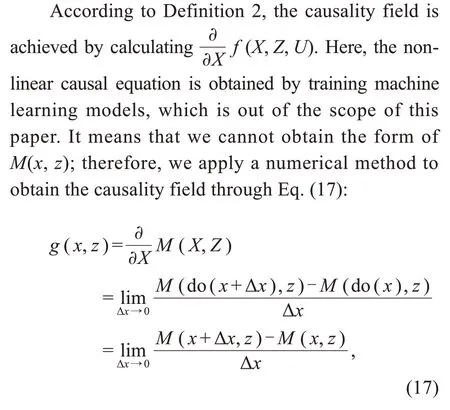
whereM(do(x)，z)represents the value ofywhen performing the interventionX=x，given the conditionZ=z.Zis the unique backdoor variable，soM(do(x)，z)=E Z[M(x，z)].

AlthoughX，Y，andZmay be continuous vari‐ables，their values are discrete in practical datasets.Thereby，for eachxandz，we can use the established model to computeg(x，z)，while ACE(X→Y)can be computed by ∑z g(x，z)P(z).

Fig.2 shows the causality field and ACE of the alcohol consumption(X)on the suicide rate(Y)with income per person(Z)as the confounding variable.From ACE，we can find that with the increase ofX，the causal effect first decreases and then increases.Besides，ACEs are larger than 0 regardless of the value ofX，which means thatXhas only a positive effect onY.This indicates that consuming alcohol can only increase the suicide rate.It seems that if the policy makers want to reduce this rate，they should strictly prohibit alcohol consumption.However，when we check the causality field，although it shows similar trends to ACE，there are still some effects that are smaller than 0 for differentZvalues;i.e.，there are negative causality field and null causality field.This means that consuming a certain amount of alcohol can sometimes reduce the suicide rate when the values ofXandZfall into the scope of the negative causality field;hence，we should allow some alcohol consump‐tion to reduce the suicide rate.

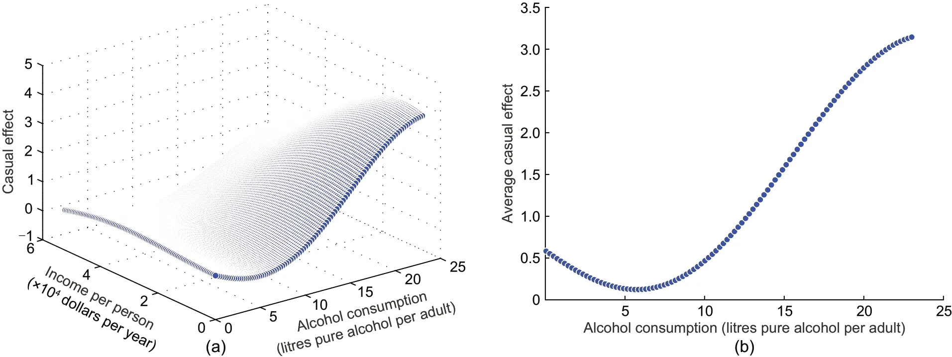
Fig.2 Causal effect of the alcohol consumption on the suicide rate with income per person as the confounding variable:(a)causality field;(b)average causal effect

To obtain the particular form of the causality field，we fit a polynomial functiong(x，z)according to these discretex，zvalues.Since the ranges ofxandzconsiderably vary，we perform normalization onxandzbefore fitting the function.The mean and stan‐dard deviation ofxare 11.5 and 6.7，respectively，while the mean and standard deviation ofzare 2.62×104and 1.51×104，respectively.Eq.(18)shows the function:

The root-mean-square error(RMSE)is 0.094.If{x，z}satisfiesg(x，z)=0，then we can obtain the null causality fieldΩ0.If{x，z}satisfiesg(x，z)＜0，then we can achieve the negative causality fieldΩ-.We can also obtain the positive causality fieldΩ+by settingg(x，z)＞0.For example，the values{-1.103，1}，{-0.8，1}，{0，1}of{X，Z}fall into the scopes of null causality field，negative causality field，and positive causality field respectively.These values are normalized，and they correspond to the original values{4.11，4.14×104}，{6.14，4.14×104}，and{11.4，4.14×104}respectively.

Figs.3a and 3b respectively show the causality field and ACE of BMI(X)on life expectancy(Y)with GDP(Z)as the confounding variable.The normal range of BMI is 18.5 to 25.We can find that，in this normal range，ACE increases with the increase of BMI.Beyond this normal range，ACE will decrease.However，if we check the SCEzfigure，we can find that when GDP is larger than a threshold，BMI has no effect on life expectancy.This means that，for lower GDP，policy makers should pay attention to BMI to increase people’s life expectancy，while for higher GDP，if they want to increase life expectancy，BMI is no longer a factor to consider.This fact could not be discovered from ACE.If polices are formed according to ACE，there will be a waste of resources.For this dataset，we do not fit functions for the unabridged form，and only estimate the causality field for some data points，asg(x，z)is too complicated.

Figs.4a and 4b respectively illustrate the causal effect and ACE of insulin(X)on diabetes(Y)with age(Z)as the confounding variable.For this dataset，Yis binary and contains only two values，namely having diabetes or not having diabetes.Therefore，we apply the softmax function to convert the output into a con‐tinuous value within the range from 0 to 1.For this dataset，the causality field and ACE show a similar trend.With the increase of insulin，the causal effect decreases regardless of age.When it is larger than a threshold，insulin has negative effect on diabetes，which means that it can prevent the onset of diabetes.When it is lower than a threshold，insulin can increase the risk of diabetes.However，there is still a small difference among different ages given the same insulin dose.It means that the threshold for insulin on diabetes varies according to age，and this variation is concealed by averaging.We can control different thresholds of insulin according to the age rather than using a fixed threshold.After fitting a polynomial function，we can obtaing(x，z)as

Fig.3 Causal effect of BMI on the life expectancy with GDP as the confounding variable:(a)causality field;(b)average causal effect

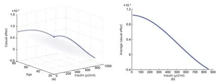
Fig.4 Causal effect of insulin on diabetes with age as the confounding variable:(a)causality field;(b)average causal effect

Subsequently，we can identify the causality fieldΩ0，Ω+，andΩ-based on this equation.

From the above three examples，we can infer that the causality field differs a lot from the average causal effect.Whenzvaries，the causal effect will change even for the samex.This inspires us that，when trying to figure out the causal effect ofXonY，we should check the confounding variableZand choose different strategies according to its value.This can be applied for various situations，e.g.，different individuals and environments.This approach could guide the individualized policy making process like precision medicine.

Notably，we have used simple confounding vari‐ables in the above three examples.In practice，it is usually difficult to determine the confounding vari‐ables.The above are just examples to illustrate the differences between the causality field and ACE.When handling complicated datasets，researchers should refer to the graph-based model，potential-outcome framework，or even deep learning based model to obtain the causality field.However，these methods are beyond the scope of this paper.

5 Conclusions

We present preliminary discussions on the problems of nonlinear causal effect calculation and the causality field，which are pivotal for solving complex practical problems.These discussions could help understand both linear and nonlinear causal relations.We expect further considerations of these problems to facilitate the research on nonlinear causal relations and their wider application.

Contributors

Aiguo WANG，Li LIU，Jiaoyun YANG，and Lian LI designed the research.Jiaoyun YANG processed the data.Aiguo WANG，Li LIU，Jiaoyun YANG，and Lian LI drafted the paper.Aiguo WANG，Li LIU，and Jiaoyun YANG revised and finalized the paper.

Compliance with ethics guidelines

Aiguo WANG，Li LIU，Jiaoyun YANG，and Lian LI declare that they have no conflict of interest.