Training time minimization for federated edge learning with optimized gradient quantization and bandwidth allocation*#

Peixi LIU，Jiamo JIANG，Guangxu ZHU，Lei CHENG，Wei JIANG，Wu LUO，Ying DU，Zhiqin WANG

1State Key Laboratory of Advanced Optical Communication Systems and Networks，Department of Electronics，Peking University，Beijing 100871，China

2China Academy of Information and Communications Technology，Beijing 100191，China

3Shenzhen Research Institute of Big Data，Shenzhen 518172，China

4Col lege of Information Science and Electronic Engineering，Zhejiang University，Hangzhou 310027，China

5Zhejiang Provincial Key Laboratory of Information Processing，Communicat i on and Networking，Hangzhou 310027，China

†E-mail:jiangjiamo@caict.ac.cn;gxzhu@sribd.cn

Abstract:Training a machine learning model with federated edge learning(FEEL)is typically time consuming due to the constrained computation power of edge devices and the limited wireless resources in edge networks.In this study，the training time minimization problem is investigated in a quantized FEEL system，where heterogeneous edge devices send quantized gradients to the edge server via orthogonal channels.In particular，a stochastic quantization scheme is adopted for compression of uploaded gradients，which can reduce the burden of per-round communication but may come at the cost of increasing the number of communication rounds.The training time is modeled by taking into account the communication time，computation time，and the number of communication rounds.Based on the proposed training time model，the intrinsic trade-offbetween the number of communication rounds and per-round latency is characterized.Specifically，we analyze the convergence behavior of the quantized FEEL in terms of the optimality gap.Furthermore，a joint data-and-model-driven fitting method is proposed to obtain the exact optimality gap，based on which the closed-form expressions for the number of communication rounds and the total training time are obtained.Constrained by the total bandwidth，the training time minimization problem is formulated as a joint quantization level and bandwidth allocation optimization problem.To this end，an algorithm based on alternating optimization is proposed，which alternatively solves the subproblem of quantization optimization through successive convex approximation and the subproblem of bandwidth allocation by bisection search.With different learning tasks and models，the validation of our analysis and the near-optimal performance of the proposed optimization algorithm are demonstrated by the simulation results.

Key words:Federated edge learning;Quantization optimization;Bandwith allocation;Training time minimization

1 Introduction

1.1 Background

The evolution of wireless networks from the first generation(1G)to the fifth generation(5G)advanced(5G-advanced)has witnessed a paradigm shift，from connecting people targeting human-type communications towards connecting intelligence targeting machine-type communications，to attain the vision of Artificial Intelligence of Things(AIoT).This has driven the rapid development of an emerging area called edge intelligence，positioned at the intersection of two disciplines，namely artificial intelligence(AI)and wireless communications(Letaief et al.，2019;Park et al.，2019).In edge intelligence，AI technologies are pushed toward the network edge so that the edge servers can quickly access real-time data generated by edge devices for fast training and real-time inference(Zhu et al.，2020b).A promising framework for distributed edge learning，called federated edge learning(FEEL)，has recently been pushed into the spotlight;it distributes the task of model training to edge devices and keeps the data locally at the edge devices to avoid data uploading and thus to preserve user privacy(Zhu et al.，2020a;Chen et al.，2021b;Liu and Simeone，2021).Specifically，a typical training process of FEEL involves multiple rounds of wireless communication between the edge server and devices.In a particular round，the edge server first broadcasts the global model under training to the edge devices for local stochastic gradient descent(SGD)execution using local data，and then the edge devices upload their local models/gradients to the edge server for aggregation and global model updating.After the convergence criterion，such as attaining a desired level of accuracy or reaching a pre-defined value of the loss，is met，the entire training process is completed，and then on-device models can be tweaked for the edge devices’personalization.

In edge networks，the computation resources of the edge devices are constrained，and the wireless resources of the network，e.g.，frequency bandwidth，are also limited;therefore，training an AI model by FEEL is usually a time-consuming and expensive task that can take anywhere from hours to weeks(Chen et al.，2021a).Hence，training time(This is also called wall-clock time in some literature(Kairouz et al.，2019;Nori et al.，2021).In this work，we use“total training time，”“training time，”and“wall-clock time”interchangeably.)minimization of AI models is one of the critical concerns in FEEL.The whole training process of FEEL typically consists of multiple communication rounds，and each round lasts a period of time consisting of computation time and communication time，which we call per-round latency.To reduce the total training time，we should not only bring down the number of communication rounds，i.e.，increase the convergence rate of the learning algorithm，but also shorten the per-round latency.Communication-efficient transmission achieved through compression is usually included into the FEEL pipeline to alleviate the transmission burden of the edge devices，and thus the per-round latency is reduced(Park et al.，2021).Two main lossy compression techniques，namely quantization and sparsification，as well as the combination of them，have been considered in the literature(Alistarh et al.，2017;Stich et al.，2018;Wangni et al.，2018;Amiri and Gündüz，2020a，2020b;Basu et al.，2020;Reisizadeh et al.，2020;Zhu et al.，2021).Specifically，in the case of quantization，the gradient vector entries are transmitted after being quantized to finite bits，instead of the full floating-point values(Alistarh et al.，2017;Reisizadeh et al.，2020;Zhu et al.，2021).Sparsification reduces the communication overhead by sending only significant entries of the gradient vector(Stich et al.，2018;Wangni et al.，2018).Although the compressed transmission can decrease the per-round latency，the lossy compression degrades the convergence speed of FEEL as well，which leads to an increase in the number of communication rounds needed to achieve a certain accuracy on a given task(Basu et al.，2020).As a result，the compression level balances the number of communication rounds and the per-round latency during minimization of the total training time in FEEL.Besides，edge devices in the edge network are usually heterogeneous，such that some of the edge devices with lower computation power become laggards in the synchronous model/gradient aggregation due to their longer computation time，which increases the per-round latency.It is necessary to consider the optimization of wireless resources over different edge devices to reduce the communication time of the lagging edge devices and compensate for the longer computation time(Dinh et al.，2021;Nguyen et al.，2021;Wan et al.，2021).With the goal of minimizing the total training time，we analyze the following question:how to balance the number of communication rounds and the per-round latency via joint quantization level and bandwidth allocation optimization in the presence of device heterogeneity.

1.2 Related works

Recently，extensive efforts have been made to minimize the total training time of FEEL by resource allocation or gradient/model compression，which fall mainly into three categories in terms of their objectives.

1.2.1 Minimization of the number of communication rounds

This is equivalent to accelerating the convergence of FEEL algorithms.Chen et al.(2021b)minimized the global loss function by optimizing the communication resources，e.g.，power and bandwidth，and the computation resources under the given perround latency constraint，and thus the convergence speed was maximized.Salehi and Hossain(2021)and Wang YM et al.(2022)considered quantization and bandwidth optimization to accelerate the algorithm convergence of FEEL with device sampling in the presence of outage probability.In Chang and Tandon(2020)，stochastic gradient quantization was adopted to compress the local gradient，and the quantization levels of each device were optimized to minimize the optimality gap under multiple-access channel capacity constraints.These efforts focused on speeding up the convergence of the FEEL algorithms，i.e.，reducing the number of communication rounds，without considering minimization of the total training time，which is a more practical and important issue in FEEL.

1.2.2 Minimization of the per-round latency

Dinh et al.(2021)and Nguyen et al.(2021)studied the trade-offbetween the per-round latency and the energy consumption by introducing a weight factor，and these two objectives tend to form a competitive interaction. Zhu et al.(2020a)analyzed the per-round latency of different multiple-access schemes in FEEL，i.e.，the proposed broadband analog aggregation(BAA)and the traditional orthogonal frequency-division multiple access(OFDMA)，and proved that the proposed BAA can significantly reduce the per-round latency compared to the traditional OFDMA.The resource allocation over each single communication round was considered in Zhu et al.(2020a)，Dinh et al.(2021)，and Nguyen et al.(2021).Nevertheless，FEEL is a long-term process consisting of many communication rounds that determine the total training time.

1.2.3 Minimization of the total training time

Wan et al.(2021)minimized the total training time by optimizing the communication and computation resource allocation;however，no compression was considered therein.Chen et al.(2021a)minimized the training time for a fixed number of communication rounds by solving a joint learning，wireless resource allocation，and device selection problem.Some other works did not minimize the training time directly，but the minimization of the loss function in a given training time was considered.For example，Nori et al.(2021)studied the communication trade-offbetween compression and local update steps in a fixed training time，but communication resource allocation was not taken into consideration.Jin et al.(2020)adopted the idea of signSGD with majority vote(Bernstein et al.，2018)and optimized the power allocations and central processing unit(CPU)frequencies under the trade-offbetween the number of communication rounds and the outage probability per communication round for a fixed training time.

Despite the above research efforts，these prior works have overlooked the inherent trade-offin minimizing the total training time of communicationefficient FEEL between the number of communication rounds and the per-round latency，which is balanced by the quantization level at the edge devices.Moreover，the communication resource allocation among different edge devices and the compression setup for minimizing the total training time of communication-efficient FEEL should be jointly considered.This thus motivates the current work.

1.3 Our contributions

This paper studies a FEEL system consisting of multiple edge devices with heterogeneous computational capabilities and one edge server for coordinating the learning process.We consider quantized FEEL，whereby a stochastic quantization scheme is adopted for updated gradient compression，which can save per-round communication cost but may come at the cost of increasing the number of communication rounds.Thus，we make a comprehensive analysis of the total training time by taking into account the communication time，computation time，and the number of communication rounds，based on which the intrinsic trade-offbetween the number of communication rounds and the per-round latency is characterized.Then，based on the analytical results，a joint quantization and bandwidth allocation optimization problem is formulated and solved.The main contributions are elaborated as follows:

1.Training time analysis in quantized FEEL

The challenge of analyzing the total training time lies mainly in estimating the number of required communication rounds for model convergence.To tackle this challenge，we analyze the convergence behavior of quantized FEEL in terms of the optimality gap and establish the expression for the minimum number of communication rounds to obtain a particular optimality gap of the loss function.However，the derived results are generally too loose to be used for further optimization.To yield an accurate estimate of the number of required communication rounds，we propose a joint data-and-model-driven fitting method to further refine and tighten the derived results.Owing to the refinement，an accurate estimate of the total training time can be attained and the trade-offbetween the number of communication rounds and the per-round latency can be better characterized.

2.Training time minimization via joint optimization of quantization and bandwidth

Next，based on the derived analytical results，we formulate the total training time minimization problem by jointly optimizing the quantization level and bandwidth allocation，subject to a maximum bandwidth constraint in the FEEL network.The problem is non-convex，and thus is challenging to solve.To tackle this challenge，we adopt the alternating optimization technique to decompose the problem into two subproblems，and each optimizes one of the two control variables with the other variable fixed.The subproblem of bandwidth allocation with a fixed quantization level can be solved by bisection search efficiently. For the subproblem of quantization optimization with bandwidth allocation fixed，an algorithm based on successive convex approximation(SCA)is proposed.

3.Performance evaluation Finally，we conduct extensive simulations to evaluate the performance of task-oriented resource allocation for quantized FEEL by considering logistic regression(convex loss function)on a synthetic dataset and a convolutional neural network(non-convex loss function)on the Canadian Institute For Advanced Research(CIFAR)-10 dataset.It is shown that the results of the proposed joint dataand-model-driven fitting method fit the curve of the actual optimality gap well.In addition，it is shown that the optimal quantization level found by solving the formulated optimization problem matches well the simulation results.The benefits of optimizing the bandwidth allocation for coping with device heterogeneity are also demonstrated.

NotationsR represents the set of real numbers.[K]denotes the set{1，2，...，K}.∅denotes the empty set.sgn(·)denotes the sign of a scalar.wTis the transpose of vectorw.∇f(w)denotes the gradient of functionfat pointw.‖w‖denotes theℓ2norm of vectorw.「x■is the ceiling operator.x～C N(0，σ2)denotes the zero-mean circularly symmetric complex Gaussian(CSCG)random variable with the variance ofσ2.

2 System model

2.1 Federated learning

We consider a quantized FEEL system consisting ofKedge devices and a single edge server，as shown in Fig.1.With the coordination of the edge server，the edge devices collaboratively train a shared model，which is represented by the parameter vectorw∈Rd，withddenoting the model size.The training process is performed to minimize the following empirical loss function:

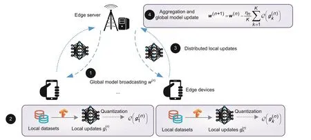
Fig.1 Quantized federated edge learning(FEEL)system with K edge devices

whereF k(w)denotes the local loss function at edge devicek，k∈[K].Suppose that devicekholds the training datasetD kwith a uniform size ofD，i.e.，|D k|=D.The local loss functionF k(w)is given by the following expression:

wheref(w;x i，y i)denotes the sample-wise loss function specified by the learning task and quantifies the training loss of modelwon the training datax iand its ground-true labely i.

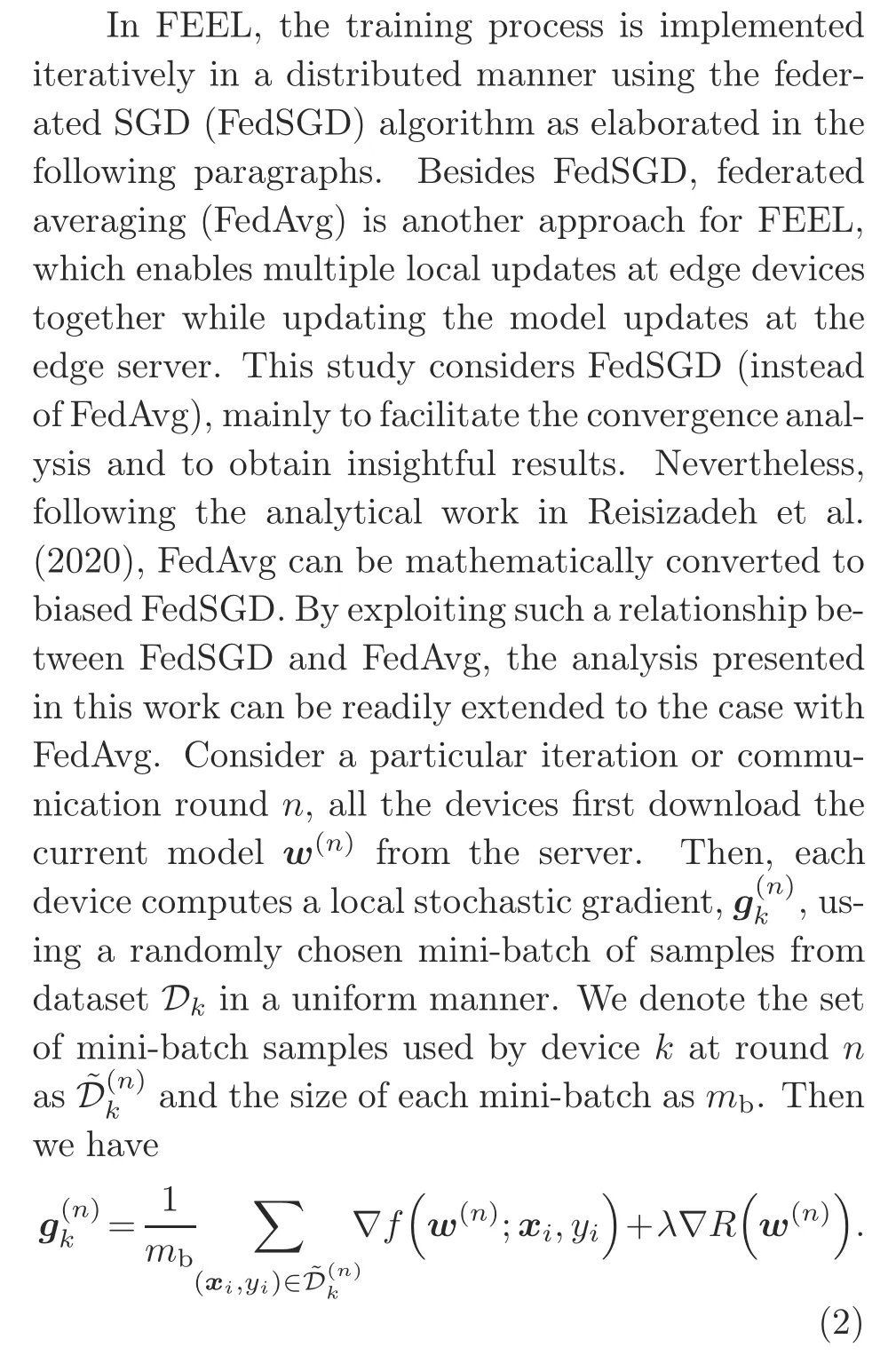
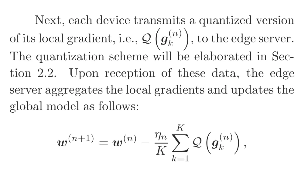
whereηndenotes the learning rate at roundn.Then the updated global model is broadcasted back to all edge devices for initializing the next round of training.The above procedure continues until the convergence criterion is met.

2.2 Stochastic quantization

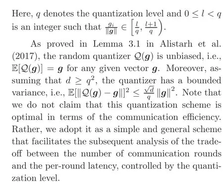
We consider a widely used stochastic quantizer for local gradient quantization(Alistarh et al.，2017).For any arbitrary vectorg∈Rd，the stochastic quantizerQ(g):Rd→Rdis defined as

where the output of quantizerQ(g)consists of three parts，i.e.，the vector norm‖g‖，the sign of each entry sgn(g i)withg idenoting theithentry ofg，and the quantization value of each entryξi(g，q).Further，the termsξi(g，q)are independent random variables defined as

2.3 Wireless transmission model

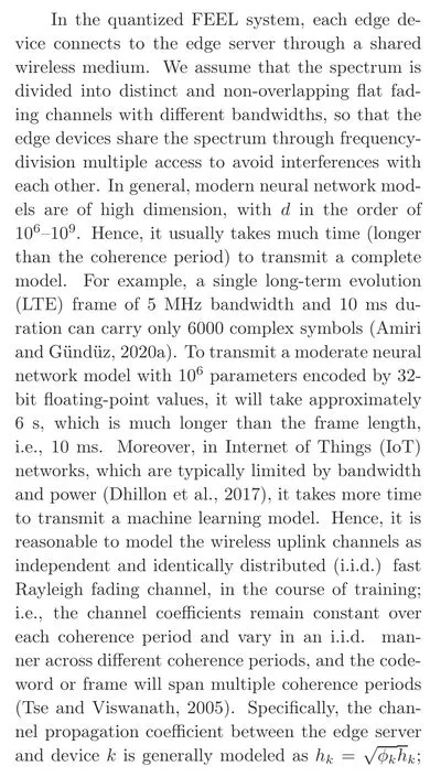
In this situation，the ergodic capacity can be assigned to the fast fading channel and achieved in practice by the interleaving technique(Tse and Viswanath，2005).The ergodic capacity of devicekis given by

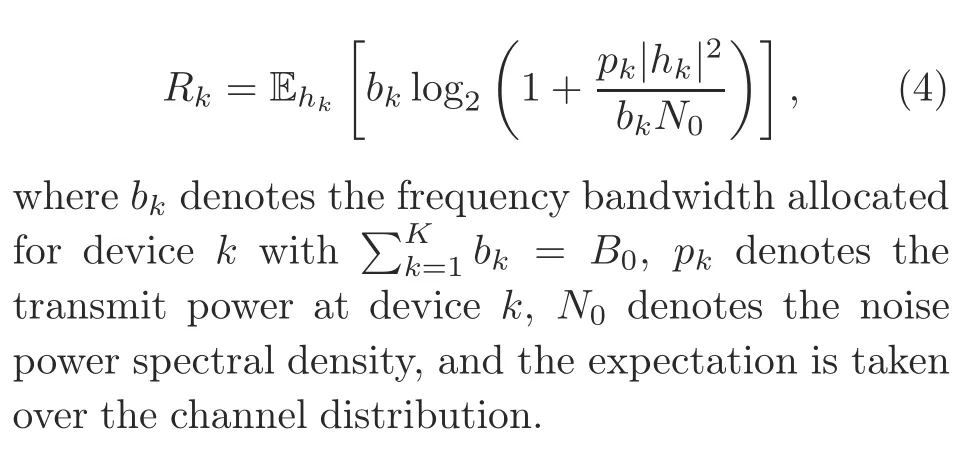
3 Training time analysis

In the following subsections，we give the expression of per-round training timeTdand obtain the minimum number of communication roundsN∈by analyzing the convergence of FEEL，which paves the way for minimizing the total training time in Section 4.

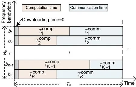
Fig.2 Computation time and communication time in one communication round of quantized FEEL

3.1 Computation time

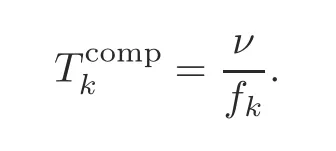
Letνdenote the number of processing cycles for one particular edge device to execute the SGD operation on one batch of samples，andf kthe CPU frequency of devicek.Accordingly，the computation time for running one-round SGD at devicekis given by the following expression(Ren et al.，2020):

3.2 Communication time

LetSdenote the number of bits for transmission after stochastic quantization.For quantizing any elementg iin gradient vectorg∈Rd，as noted in Eq.(2)，we need to encode the vector norm‖g‖，the element-wise sign sgn(g i)，and the normalized quantization valueξi(g，q)into bits.Particularly，it takes one bit to encode each of the sgn(g i).Sinceξi(g，q)takes value from{0，1/q，2/q，...，1}，it takes at most log2(1+q)bits to encode eachξi(g，q)(Cover and Thomas，2006).Since each vector containsdentries，it takes totally(1+log2q)dbits to encode these two parts.By contrast，the overhead in encoding the single scalar vector norm‖g‖is typically negligible for large models of sized(Shlezinger et al.，2021).To facilitate subsequent analysis，for larged，we approximateSusing the following expression:

The communication delay in one round is

whereR kis the ergodic capacity defined in Eq.(4).

3.3 Minimum number of communication rounds

In this subsection，we deriveN∈by analyzing the convergence of quantized FEEL.To this end，we make the following assumptions on the local loss functions{F k(w)}:

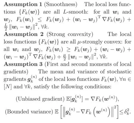
Assumptions 1 and 2 on local loss functions are standard，and they can be satisfied by many typical learning models，such as logistic regression，linear regression，and softmax classifier.Assumption 3 is general enough to cope with both i.i.d.and non-i.i.d.data distributions across edge devices，following the work in Li et al.(2020)，Luo et al.(2021)，and Salehi and Hossain(2021).Under Assumptions 1-3，the convergence rate of quantized FEEL is established in the following theorem:

Theorem 1Consider a quantized FEEL system with fixed quantization levelq≥2.The optimality gap of the loss function afterNcommunication rounds is upper bounded by

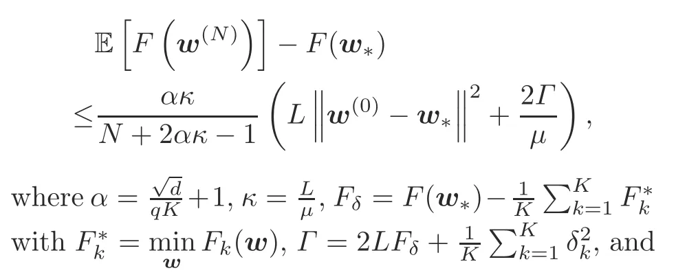
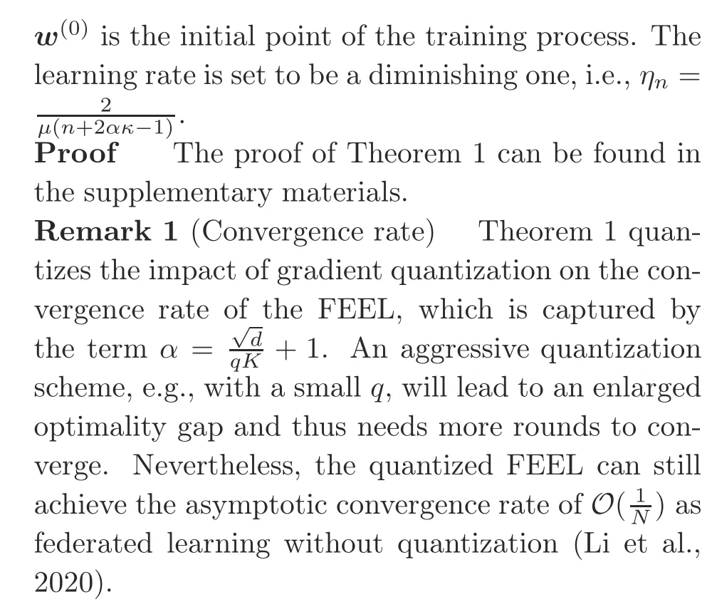
Although we can readily establish a bound onN∈based on Theorem 1 and apply this bound for subsequent resource optimization as was done in prior works，e.g.，Wang SQ et al.(2019)and Luo et al.(2021)，such an approach has two key drawbacks:First，the gap between the derived bound and its true value could be large as several relaxations are made in deriving the bound.Thus，ignoring the gap may lead to a highly suboptimal solution in the subsequent resource optimization stage.Second，even if we adopt the upper bound and ignore the effects of the gap，it is still difficult to obtain the exact value of the upper bound，since it involves calculating a bunch of data-and model-related parameters，such asμ，L，Fδ，w*，andΓ.

To address the above issues，we propose a joint data-and-model-driven fitting approach，which uses a small number of pre-training rounds to yield a good estimate of the optimality gap based on the bound derived in Theorem 1.To this end，we first denote the upper bound function derived in Theorem 1 as follows:

Before we derive the tight estimate of the optimality gap，it is first observed that the upper bound functionˆU(N)satisfies the following properties:

(1)ˆU(N)is a decreasing function ofN，and it converges to zero at a rate of

(2)ˆU(N)has a fractional structure，where the numerator and denominator are both linear increasing functions ofα.

We assume that the ground-true optimality gap follows the same properties as its upper boundˆU(N).Based on the above assumption，the exact optimality gap can be well estimated by the following function:

whereA＞0，B＞0，C≥0，andD≥0 are the tuning parameters to be fitted and implicitly related to parameters such asμ，L，Fδ，andΓ.It can be seen thatU(N)generalizes all the functions that satisfy the two properties mentioned above.

Next，we apply a joint data-and-model-driven fitting method to fit the values of the tuning parameters as follows:First，we randomly choose two quantization levels，sayq1andq2，and run the quantized FEEL withq1andq2，separately，from an initial modelw0.Then，we sample the value of loss at each round until the number of communication rounds reaches a pre-defined value~N.The corresponding loss values are denoted asF i，n(i∈{1，2}，n∈[1，~N])for roundnwhen the quantization level isq i.According to Eq.(8)，we have

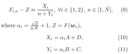
Then we aim to find the proper values ofX i，Y i，andZto fit expression(9)well.The method we choose is to solve the following nonlinear regression problem:

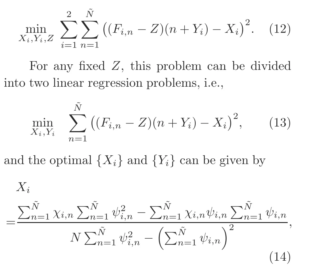
whereχi，n=(F i，n-Z)nandψi，n=F i，n-Z.Hence，problem(12)can be solved by a one-dimensional search ofZ.Since the computations in Eqs.(14)and(15)involve only limited algebraic operations，the computation time for solving problem(12)is negligible compared with the time needed in the whole training process.With{X i}and{Y i}at hand，A，B，C，andDcan be obtained from Eqs.(10)and(11)as follows:

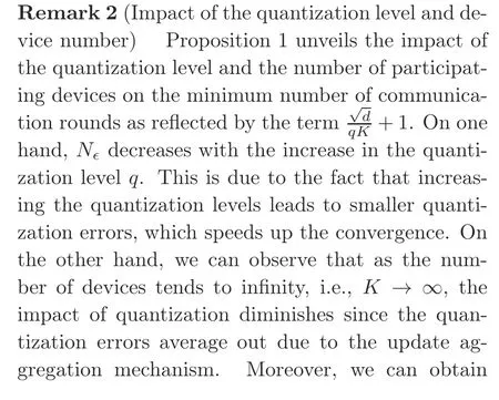
Based on the estimated optimality gap in Eq.(8)with the well-fitted parameters，we can deriveN∈in the following proposition:

Proposition 1In the quantized FEEL system，the minimum number of communication rounds needed to achieve the∈-optimality gap is given by

ProofBy setting the fitted optimality gap in Eq.(8)to be less than∈，i.e.，U(N)≤∈，and respecting the fact that the minimum number of communication rounds should be an integer，we obtain Eq.(16).

4 Training time minimization

In this section，we aim to jointly optimize the quantization level and bandwidth allocation by minimizing the training time defined in Eq.(5)to achieve an∈-optimality gap.

4.1 Problem formulation

The training time minimization problem is mathematically formulated as follows:

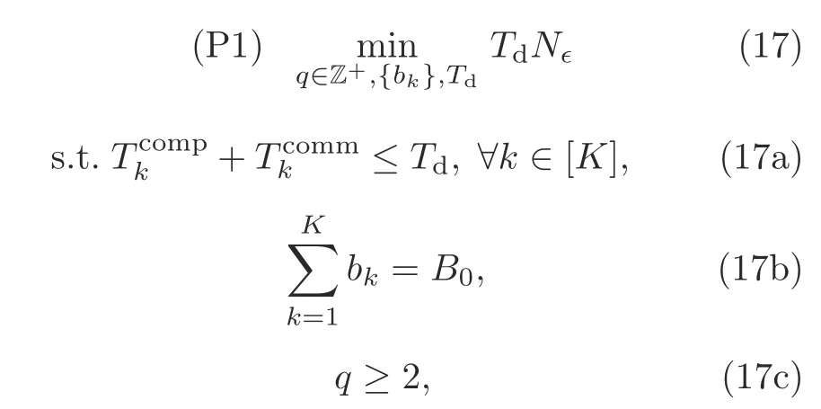
where the objective function in problem(17)is the total training time needed to achieve the∈-optimality gap.Constraint(17a)indicates that the training time of each device per communication round cannot exceed the delay requirementTd.Constraint(17b)means that the total bandwidth allocated to all the devices isB0.The constraint on the quantization levelqis described by constraint(17c).

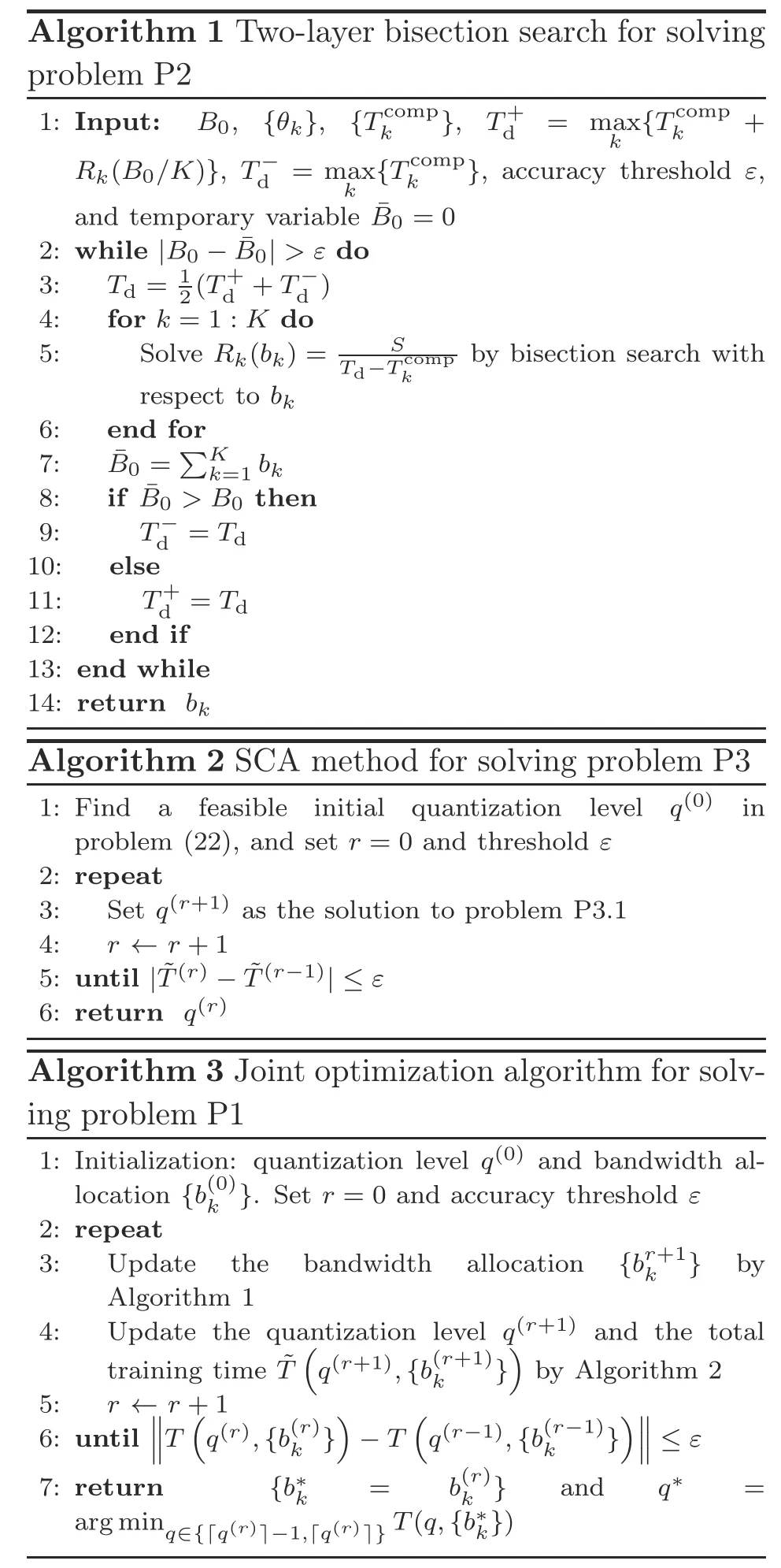
The objective function in problem(17)is complicated due to the coupling of the control variablesTdandq.Moreover，qcan take values only from positive integers.Therefore，problem P1 is non-convex，and is challenging to solve optimally.To yield a good solution to problem P1，we divide it into two subproblems:One is to find the optimal bandwidth allocation{b k}andTdwith fixed quantization levelq，and the other is to find the optimal quantization levelqwith fixed bandwidth allocation{b k}andTd.We find that the first subproblem can be solved optimally and efficiently with a unique solution，and the second one can be transformed into a non-convex problem that can be solved by the method of SCA(Razaviyayn，2014).Then，by alternatively solving each subproblem，we can obtain good sub-optimal solutions for joint quantization level and bandwidth allocation optimization.

Remark 3(Trade-offbetween the minimum number of communication rounds and the per-round latency)As noted in Remark 2，the minimum number of communication roundsN∈can be reduced by increasing the quantization levelq，but at a cost of increasing the per-round latency.Therefore，when minimizing the total training time，there exists a fundamental trade-offbetween reducing the minimum number of communication rounds and suppressing the per-round latency.The trade-offis manipulated by the setting of the quantization levelq.

Remark 4(Resource allocation over heterogeneous devices in FEEL) The computation time of the devices varies due to their heterogeneous computation capacities.To enforce the per-round latency constraint，a wider frequency bandwidth should be allocated to the devices with lower computation power to compensate for the long computation time with short communication time，and vice versa.Hence，the bandwidth allocation among the devices should jointly account for the channel condition and the computation resources，which is in sharp contrast to the classic bandwidth allocation problem accounting for only the channel condition，e.g.，the problem in Gong et al.(2011).

4.2 Bandwidth allocation optimization

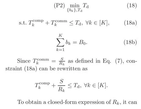
SinceN∈is independent of{b k}andTd，problem(17)under a fixed quantization levelqis reduced to

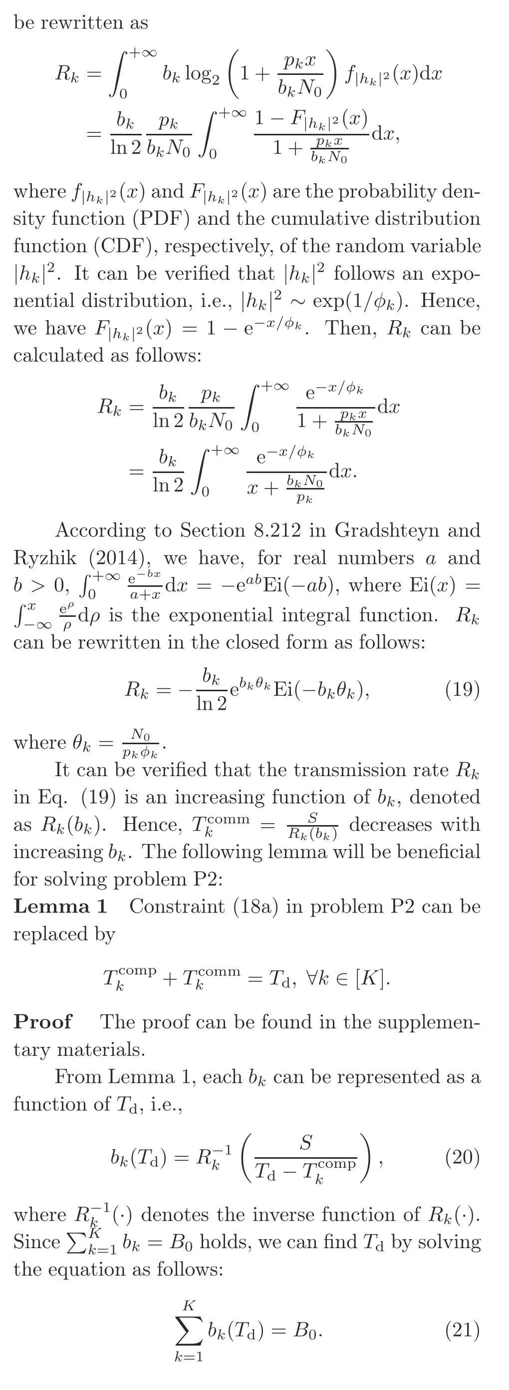
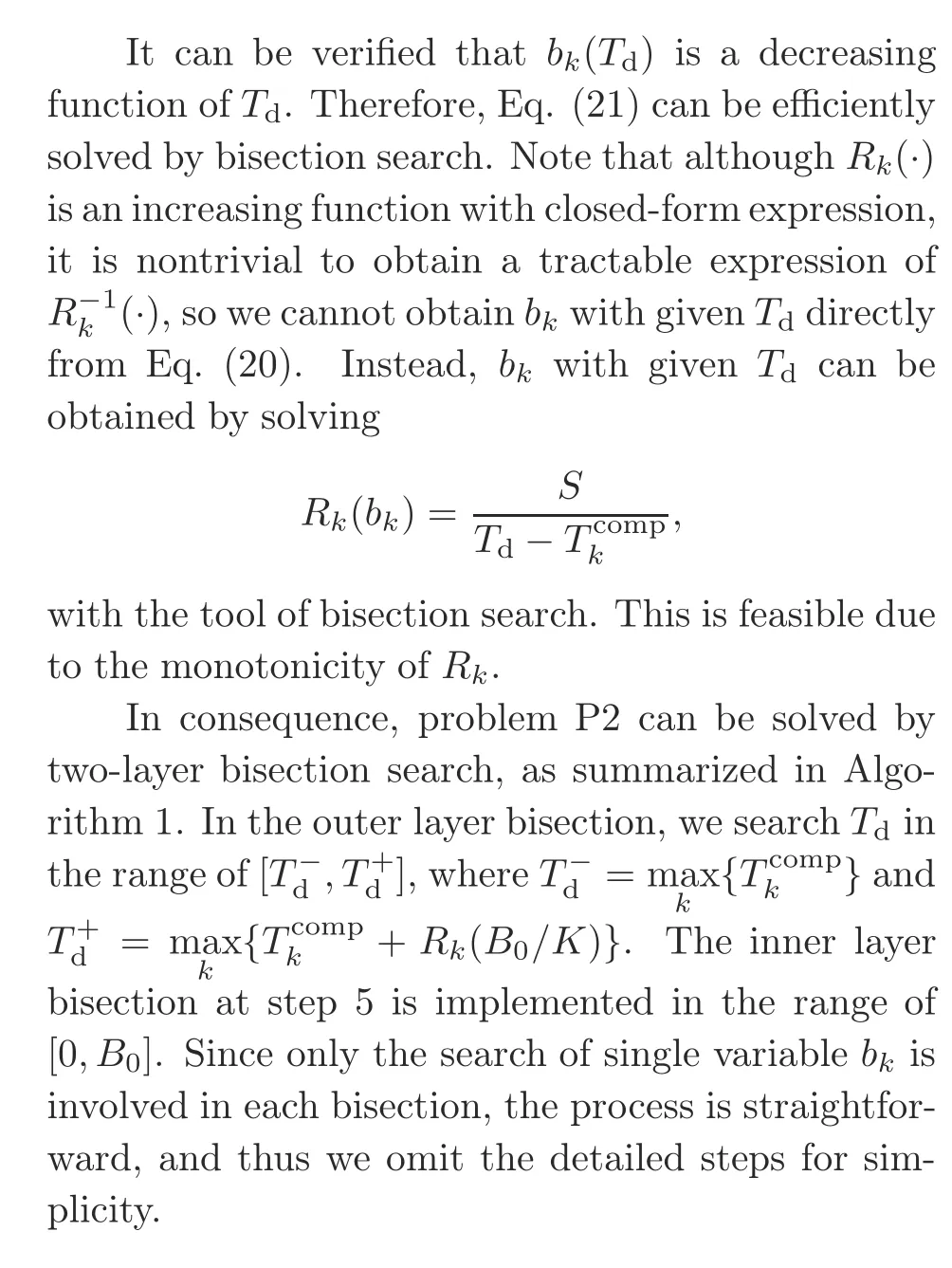
4.3 Quantization level optimization

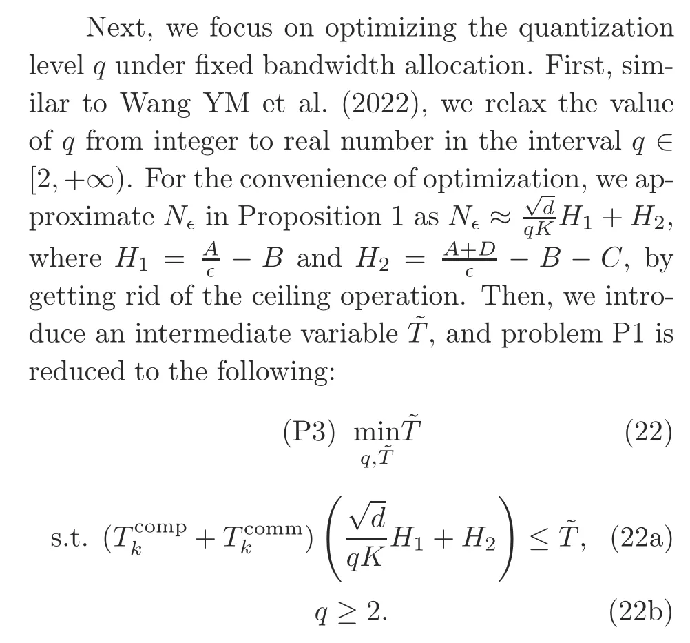
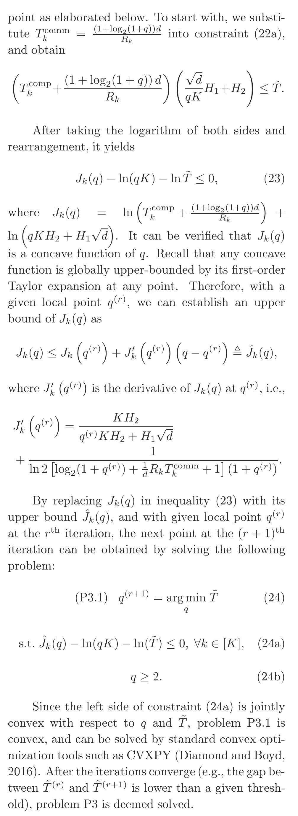
Problem P3 is non-convex due to the nonconvexity of constraint(22a).To tackle this problem，the SCA technique can be applied to obtain a stationary point(Razaviyayn，2014).The above procedure is summarized in Algorithm 2.The key idea is that at each iteration，the original problem is approximated by a tractable convex one at a given local

4.4 Joint optimization algorithm

Since the unique solution to problem P2 can be obtained by Algorithm 1 and a stationary point of problem P3 can be reached by Algorithm 2，the sub-optimal bandwidth allocation and quantization level can be jointly obtained by alternately solving problems P2 and P3，which is summarized in Algorithm 3.It can be verified that the sub-optimal solution from Algorithm 3 is a stationary point of the original problem P1.

Note that solving problem P1 may lead to a non-integerq，and thus we need a further rounding technique to yield an integerqfor practical implementation.One possible rounding technique is discussed as follows:We denoteT(q，{b k})as the total training time in problem P1 whenqand{b k}are substituted.After finding the optimized quantization leveland the optimal bandwidth allocationthe final quantization levelq*is obtained as

Algorithm 1 Two-layer bisection search for solving problem P2 1:Input: B0，{θk}，{T comp k }，T+d =max R k(B0/K)}，Td=max k{T comp k +k{T comp k }，accuracy thresholdε，and temporary variable¯B0=0 2:while|B0-¯B0|＞εdo 3: T d=1 2(T+d+Td)4: for k=1:K do 5: Solve R k(b k)= S by bisection search with respect to b k 6: end for 7: ¯B0=∑Kk=1 b k T d-T comp k 8: if¯B0＞B0 then 9: Td=T d 10: else 11: T+d=T d 12: end if 13:end while 14:return b k Algorithm 2 SCA method for solving problem P3 1:Find a feasible initial quantization level q(0) in problem(22)，and set r=0 and thresholdε 2:repeat 3: Set q(r+1)as the solution to problem P3.1 4: r←r+1 5:until|˜T(r)-˜T(r-1)|≤ε 6:return q(r)Algorithm 3 Joint optimization algorithm for solving problem P1 1:Initialization:quantization level q(0)and bandwidth allocation{b(0)k}.Set r=0 and accuracy thresholdε 2:repeat 3: Update the bandwidth allocation {b r+1 k } by Algorithm 1 4: Update the quantization level q(r+1)and the total training time˜T（q(r+1)，{b(r+1)k }）by Algorithm 2 5: r←r+1 6:until）■■■≤ε 7:return {b*k = b(r)k} and q* =arg min q∈{「q(r)■-1，「q(r)■}T(q，{b*k})■■■T（q(r)，{b(r)k}）（-T q(r-1)，{b(r-1)k }

5 Simulation evaluation

In this section，we provide numerical results of two simulations under different wireless communication scenarios and learning tasks，in which the real system’s heterogeneity is captured，to examine our theoretical results.In simulation 1，we consider a learning task with a strongly convex loss function and a training model of small size.In simulation 2，to stretch the theory，we consider a learning task with a non-convex loss function and a training model of large size.Although our analysis is developed based on the assumption of strongly convex loss functions，we show that the proposed algorithm can work well in the case of non-convex loss functions.Both simulations are implemented by PyTorch using Python 3.8 on a Linux server with one NVIDIAR○GeForceR○RTX 3090 graphics processing unit(GPU)24 GB and one IntelXeonGold 5218 CPU.

5.1 Setup

1.FEEL system

We consider a FEEL system with an edge server covering a circular area ofr=500 m.Within this area，K=6 edge devices are placed randomly and distributed uniformly over the circular area with the exclusion of a central disk ofrd=100 m.The transmit power of each device is 1 dBm.To expose the heterogeneity of the edge devices，the CPUfrequency of each device is assumed to be uniformly distributed from 100 MHz to 1 GHz.The number of processing cycles of devicekfor executing the SGD operation on one batch of samples isν=108in simulation 1 andν=2.5×1010in simulation 2.

2.Wireless propagation

The large-scale propagation coefficient in decibels from devicekto the edge server is modeled as[φk]dB=[PLk]dB+[ζk]dB，where[PLk]dB=128.1+37.6 lg distk(distkis the distance in kilometer)is the path loss in decibels，and[ζk]dBis the shadow fading in decibels(Yang et al.，2021).In this simulation，[ζk]dBis a Gauss-distributed random variable with mean zero and variance=8 decibels.The noise power spectral density isN0=-174 dBm/Hz，and the total bandwidth isB0=10 KHz(Dhillon et al.，2017).All the simulation parameters are summarized in Table S1 in the supplementary materials.

3.Learning tasks and models

In simulation 1，we consider theℓ2regularized logistic regression task on synthetic data(Wangni et al.，2018).The local loss function in Eq.(1)at devicekis given by

wherex i∈Rdandy i∈{-1，1}.Theℓ2regularization parameterλis set toλ=10-6.It can be verified that the local loss functionF k(w)is smooth and strongly convex.Each data sample(x i，y i)is generated in four steps as follows:

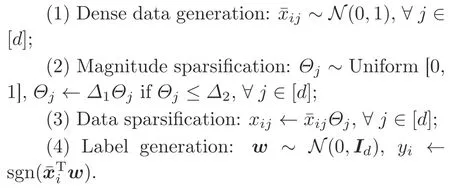
Note that the parametersΔ1andΔ2control the sparsity of data points and the gradients(Wangni et al.，2018).From our simulations，the effect of stochastic quantization on SGD convergence depends heavily on the sparsity structure of the gradients.Therefore，we choose this dataset in simulation 1 to better validate our theoretical results.Moreover，to the best of our knowledge，how the sparsity structure of the gradients affects the learning algorithm that uses stochastic quantization as the compression scheme has not been revealed in the literature，and it is an interesting topic but beyond the scope of this work.The parametersΔ1andΔ2are set to 0.9 and 0.25 in this simulation，respectively.Moreover，the dimension of each data point is set tod=1024.Hence，the model contains 1024 parameters in total.We generate 48 000 data points for training and 12 000 data points for validation.

In simulation 2，we consider the learning task of image classification using the well-known CIFAR-10 dataset，which consists of 50 000 training images and 10 000 validation images in 10 categories of colorful objectives such as airplanes and cars. ResNet-20(269 722 parameters in total)with batch normalization(The implementation of ResNet-20 follows this GitHub repository https://github.com/hclhkbu/GaussianK-SGD(Shi et al.，2019))is applied as the classifier model(He et al.，2016).

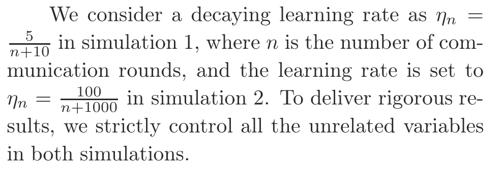
4.Training and optimization parameters

5.2 Results of simulation 1

5.2.1 Estimation of data-related parameters

In the optimization in Section 4.3，we need to obtain the values ofH1andH2using the proposed joint data-and-model-driven fitting method in Section 3.3.With the joint data-and-model-driven fitting method，for any given two quantization levelsq1andq2，and the threshold of loss optimality gap upper bound∈，we can obtain the estimates ofH1andH2，which are used in Algorithm 3.Moreover，the optimal loss value can be obtained by the estimate ofZin Eq.(9)，i.e.，F(w*)≈Z≈0.247.The threshold of the loss optimality gap upper bound is set to∈=0.012.One can choose any combination ofq1andq2to implement the estimation in theory.As a reminder to the readers，however，in our experience，the combination ofq1andq2with a large difference leads to better estimation accuracy.In our results，we choose(q1，q2)=(4，6)in the joint data-andmodel-driven fitting method and obtainH1≈43.01 andH2≈48.79.To show the robustness of our estimation method，we plot the fitted loss function and the actual loss values when(q1，q2)=(4，6)and(q1，q2)=(8，16)，as shown in Fig.3，and we can see that the fitted loss function fits the actual loss well.

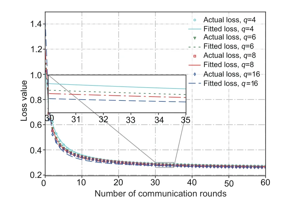
Fig.3 Robustness of the joint data-and-model-driven fitting method(the fitted loss function and the actual loss vs.the number of communication rounds when the quantization levels are set as q1 and q2)

5.2.2 Optimization of the quantization level

Fig.4 plots the total training time vs.quantization level in simulation 1 when the bandwidth allocation is the optimal.We run the same training process at least five times on each quantization level.Fig.4 shows that there exists an optimal quantization level that minimizes the total training time.Recall the facts from Section 3 that the total training time is given byT=N∈Tdand thatN∈is a decreasing function of the quantization levelq，whileTdis an increasing function ofq.In other words，Fig.4 demonstrates the trade-offbetween the total number of the communication roundsN∈and per-round latencyTdin the FEEL system.Moreover，it can be observed from the figure that the optimal quantization level obtained in theory from Algorithm 3 in Section 4 matches the results of the simulation，which confirms the validity of our proposed algorithm.From Fig.S1 in the supplementary materials，it can be observed that the training loss of the optimal quantization level under the optimal bandwidth allocation reaches the predefined threshold in a short time.

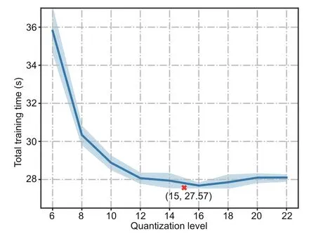
Fig.4 Total training time vs.the quantization level q in simulation 1 when the bandwidth allocation is optimal(The point with the optimal quantization level and the corresponding training time from Algorithm 3 in theory is annotated by“x”)

5.2.3 Optimization of bandwidth

Fig.S1 depicts the comparison between the schemes with the optimal and equal bandwidth allocation in terms of the loss optimality gap and test accuracy.We can observe that the scheme with the optimal bandwidth allocation can reach the predefined threshold and obtain higher test accuracy in a shorter time.This indicates that our bandwidth allocation algorithm is effective and necessary in the FEEL system.To show how the heterogeneous computation power of edge devices affects the communication resource allocation，we present the CPU frequency of each edge device and its corresponding optimal allocated bandwidth in Fig.5.It can be observed that the edge devices with a lower CPU frequency will be allocated with a larger bandwidth，which in spirit has similarity to the well-known phenomenon of“water-filling”in the problem of power allocation in wireless communication(Gong et al.，2011).

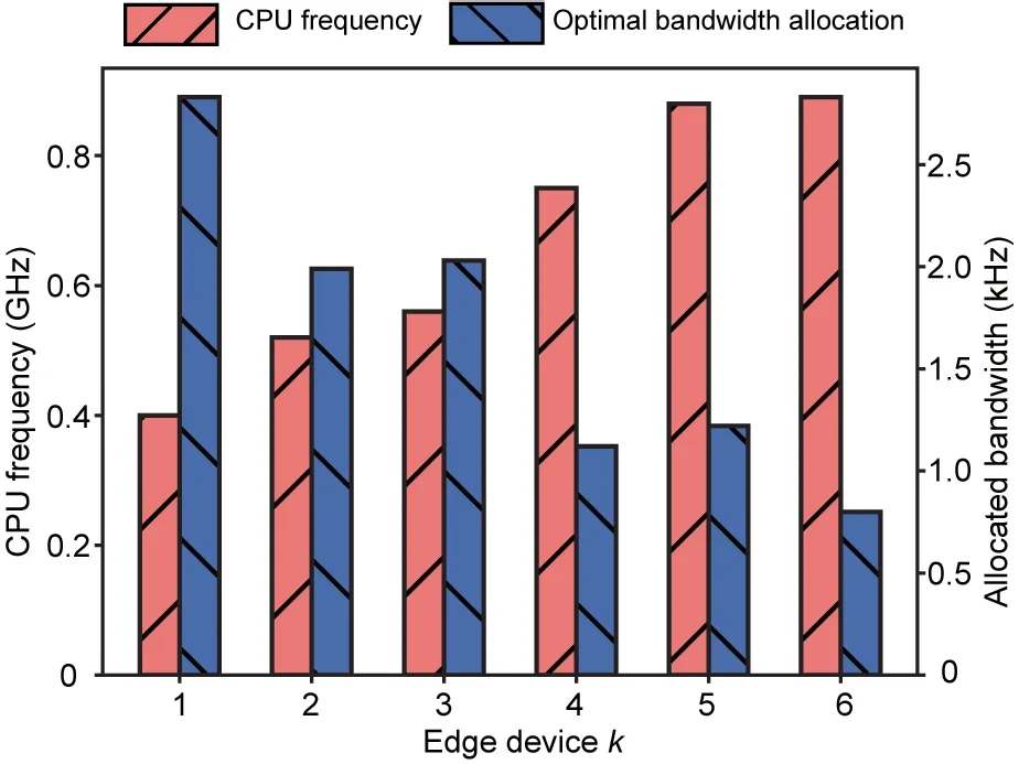
Fig.5 Optimal bandwidth allocation(bars on the right)and CPU frequency(bars on the left)of each edge device in simulation 1

5.3 Results of simulation 2

We conduct simulation 2 to evaluate our method and algorithm on the learning model with a nonconvex loss function.In this simulation，we choose(q1，q2)=(15，20)and obtainH1≈96.26 andH2≈808.53 by our joint data-and-model-driven fitting method.The threshold of the upper bound of the loss optimality gap is set to∈=0.22.Fig.6 shows the total training time vs.the quantization level during the simulation when the bandwidth allocation is optimal.Fig.S2 in the supplementary materials shows the optimality gap and test accuracy vs.training time in simulation 2 with different quantization levels and bandwidth allocations.We can obtain similar observations from Fig.6 and Fig.S2 to those in simulation 1，which reveals that our method and algorithm work well in the non-convex setting，although they are derived under a strongly convex setting.

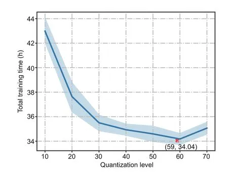
Fig.6 Total training time vs.quantization level q in simulation 2 when the bandwidth allocation is optimal(The point with the optimal quantization level and the corresponding training time from Algorithm 3 in theory is annotated by“x”)

6 Conclusions

In this study，we studied the minimization of training time for quantized FEEL with optimized quantization level and bandwidth allocation.On the basis of the convergence analysis of quantized FEEL and our proposed joint data-and-model-driven fitting method，we derived the closed-form expression of the total training time and characterized the trade-offbetween the number of communication rounds and per-round latency，which is governed by the quantization level.Next，we minimized the total training time by optimizing the quantization level and bandwidth allocation，for which high-quality nearoptimal solutions were obtained by alternating optimization.The theoretical results developed can be used to guide system optimization and contribute to the understanding of how a wireless communication system can properly coordinate resources to accomplish learning tasks.This also opens several directions for further research.One future research direction is to implement device sampling in quantized FEEL，in which how the bandwidth is allocated to minimize the training time is completely a different story.Another direction is to consider error compensation in quantized FEEL to mitigate the effects of compression errors.

Contributors

Peixi LIU，Jiamo JIANG，Guangxu ZHU，Wei JIANG，and Wu LUO designed the research.Guangxu ZHU，Wei JIANG，and Wu LUO supervised the research.Peixi LIU and Guangxu ZHU implemented the simulations.Peixi LIU drafted the paper.Jiamo JIANG and Guangxu ZHU helped organize the paper. Lei CHENG，Ying DU，and Zhiqin WANG revised and finalized the paper.

Compliance with ethics guidelines

Peixi LIU，Jiamo JIANG，Guangxu ZHU，Lei CHENG，Wei JIANG，Wu LUO，Ying DU，and Zhiqin WANG declare that they have no conflict of interest.

List of supplementary materials

Proof S1 Proof of Theorem 1

Proof S2 Proof of Lemma 1

Table S1 Simulation parameters

Fig.S1 Optimality gap and test accuracy in simulation 1

Fig.S2 Optimality gap and test accuracy in simulation 2