
Diagnostic Quantification of the Cloud Water Resource in China during 2000–2019
2022-05-07 07:06MiaoCAIYuquanZHOUJianzhaoLIUYahuiTANGChaoTANJunjieZHAOandJianjunOU
Miao CAI, Yuquan ZHOU*, Jianzhao LIU, Yahui TANG, Chao TAN, Junjie ZHAO, and Jianjun OU
1 CMA Key Laboratory for Cloud Physics, Weather Modification Center, China Meteorological Administration (CMA), Beijing 100081
2 Key Laboratory of Wetland Ecology and Environment, Northeast Institute of Geography and Agroecology,Chinese Academy of Sciences, Changchun 130102
3 University of Chinese Academy of Sciences, Beijing 100049
4 Meteorological Disaster Prevention Technology Center of Shanxi, Taiyuan 030032
5 Shanghai By Weather Technology Co., Shanghai 201306
ABSTRACT By using the diagnostic quantification method for cloud water resource (CWR), the three-dimensional (3D) cloud fields of 1° × 1° resolution during 2000–2019 in China are firstly obtained based on the NCEP reanalysis data and related satellite data. Then, combined with the Global Precipitation Climatology Project (GPCP) products, a 1° × 1°gridded CWR dataset of China in recent 20 years is established. On this basis, the monthly and annual CWR and related variables in China and its six weather modification operation sub-regions are obtained, and the CWR characteristics in different regions are analyzed finally. The results show that in the past 20 years, the annual total amount of atmospheric hydrometeors (GMh) and water vapor (GMv) in the Chinese mainland are about 838.1 and 3835.9 mm,respectively. After deducting the annual mean precipitation of China (Ps, 661.7 mm), the annual CWR is about 176.4 mm. Among the six sub-regions, the southeast region has the largest amount of cloud condensation (Cvh) and precipitation, leading to the largest GMh and CWR there. In contrast, the annual Ps, GMh, and CWR are all the least in the northwest region. Furthermore, the monthly and interannual variation trends of Ps, Cvh, and GMh in different regions are identical, and the evolution characteristics of CWR are also consistent with the hydrometeor inflow (Qhi). For the north, northwest, and northeast regions, in spring and autumn the precipitation efficiency of hydrometeors (PEh) is not high (20%–60%), the renewal time of hydrometeors (RTh) is relatively long (5–25 h), and GMh is relatively high.Therefore, there is great potential for the development of CWR through artificial precipitation enhancement (APE).For the central region, spring, autumn, and winter are suitable seasons for CWR development. For the southeast and southwest regions, Ps and PEh in summer are so high that the development of CWR should be avoided. For different spatial scales, there are significant differences in the characteristics of CWR.
Key words: cloud water resource (CWR), diagnostic quantification, weather modification regions, monthly and annual variation, development characteristics
1. Introduction
The shortage of freshwater resources is a worldwide problem, which is even more serious in China, where the per capita water resources are less than a quarter of the world average. Especially in the vast arid and semi-arid regions of the western and northern China, the lack of freshwater resources has seriously hindered the social and economic development. Atmospheric precipitation,the main source of river runoff and shallow groundwater,can be used directly by humans. Water substances in the atmosphere include water vapor and hydrometeors (in solid and liquid phases, collectively defined as cloud water). The amount of water vapor is much larger than that of cloud water, and there are long-term observational data on water vapor. Therefore, the previous studies on the water cycle and water resources in the atmosphere mainly focused on water vapor. Using radio sounding observations, ground observations, and atmospheric reanalysis data, scholars have accumulated plentiful research results on the content of water vapor in the atmosphere and its distribution characteristics, the characteristics of water vapor transport and its relationship with precipitation, and the characteristics of water vapor budgets. In terms of the water vapor content and its budget in the Chinese mainland, researchers used the radiosonde observation records to calculate the water vapor content over the Chinese mainland, and analyzed its spatial distribution and temporal variations (Cheng and Yang,1962; Zou and Liu, 1981; Liu, 1984; Sun, 1987; Wang and Liu, 1993). Xu (1957, 1958), Lu and Gao (1984), Liu and Zhou (1985), Liu and Cui (1991), Shen et al. (2010),and Sun et al. (2020) have studied the characteristics of water vapor transportation in China. In addition, based on sounding observations and atmospheric reanalysis data, Wang et al. (2003), Zhao et al. (2006), Zhang et al.(2008), Yang et al. (2010), Zhou et al. (2010), Zhou et al.(2012), Xie et al. (2014), Hu et al. (2015), and He et al.(2020) have analyzed the characteristics of physical variables, such as water vapor content, water vapor flux, and water vapor flux divergence, in the atmosphere in different provinces, regions, and river basins.
In the atmospheric water cycle, the precipitation cannot be directly formed from water vapor. At first, the water vapor needs to be transformed into hydrometeors through phase transformation. Then, hydrometeors grow larger through cloud physical processes and finally fall to the ground as surface precipitation to supplement land water resources. Consequently, the study of atmospheric hydrometeors (cloud water) is critical. However, due to the complexity of the cloud macro- and micro-structures and the difficulty of observation, the observational researches on the cloud process and cloud field (hydrometeors), as well as the characteristics of atmospheric hydrometeor budget and cycle in the atmospheric water cycle,are quite insufficient. Previous studies (Chen et al., 2005;Zhang et al., 2006; Li et al., 2008; Li et al., 2015) mostly focused on the spatiotemporal distribution characteristics of the cloud water path (CWP) in different regions based on satellite retrieval cloud products, such as the International Satellite Cloud Climatology Project (ISCCP;Rossow and Schiffer, 1991), the NASA Clouds and the Earth’s Radiant Energy System Experiment (CERES;Wong et al., 2000; Chambers et al., 2002; Minnis et al.,2020), and the Moderate Resolution Imaging Spectroradiometer (MODIS; Ackerman et al., 2008). In these studies, CWP, i.e., the integrated mass of atmospheric hydrometeors, is generally regarded as the cloud water resource (CWR). But in fact, CWP is just a small part of CWR.
Based on the atmospheric water cycle process and the atmospheric water material balance equations, Zhou et al.(2020) presented a total of 16 component items of water vapor, hydrometeors, and total atmospheric water material(the sum of water vapor and hydrometeors) including the instantaneous/state quantities, the advection items, and the source/sink items. Furthermore, the definitions and calculation formulas of 12 characteristic quantities are proposed, such as CWR, the total amount of various atmospheric water substances, and their precipitation efficiency and renewal time. In order to quantify the CWR in a specific area and time period, Cai et al. (2020) established a diagnostic quantification method of CWR based on observations (CWR-DQ). First, water vapor and wind fields are extracted from the reanalysis products (e.g., the NCEP/NCAR reanalysis data), and precipitation is obtained directly from the surface station and/or satellite observations. For the calculation of state quantities and advection terms of hydrometeors, the acquirement of three-dimensional (3D) cloud fields (cloud fraction and cloud water content) is difficult, as routine observations of the time-varying 3D cloud fields are not available. To solve this problem, they established the relative humidity threshold to identify the cloud area and the profile of cloud water content with temperature through satellite observations. Then, the diagnosis of the 3D cloud fields is realized, and the spatial distribution of cloud water content is obtained. On this basis, the calculation of CWR and its related quantities can be realized. Meanwhile, based on a cloud-resolving model, which can describe the cloud microphysical processes completely and precisely, Zhou et al. (2020) and Cai et al. (2020) established a numerical quantification method of CWR(CWR-NQ). Through the application and comparative analysis of two typical months in spring and summer in North China, the rationality of the two sets of quantification methods and results are verified, and the CWR characteristics in the 1° × 1° grids of North China and the whole region are preliminarily analyzed.
In previous studies, there are many results on the water vapor content and its budget and circulation, but the researches on the budget and circulation of hydrometeors and CWR are rare. Zhou et al. (2020) just studied the characteristics of CWR in two typical months in North China. Overall, the research on climatic characteristics of CWR in China has not yet started. From the perspective of disaster prevention and protection of water resources, China attaches great importance to the development of CWR through artificial precipitation (snow)enhancement. In order to reasonably plan and carry out the long-term national weather modification operation, it is necessary to conduct a scientific quantification of CWR in China, and to understand its spatiotemporal distribution and evolution characteristics.
In this study, we firstly obtain the 3D cloud field distribution in China with a resolution of 1° × 1° from 2000 to 2019 based on the 3D cloud field diagnosis method established by Cai et al. (2020). Then, combining with atmospheric reanalysis data and precipitation products, we realize the diagnostic quantification of CWR on 1° × 1°grid in China from 2000 to 2019 according to the CWRDQ method. On this basis, we obtain the long-term results of CWR and its related physical quantities in China and different sub-regions through the spatiotemporal integration process. Finally, a detailed analysis of the characteristics and evolution of CWR in China and different weather modification sub-regions is conducted, so as to lay the foundation for better CWR development and utilization.
2. CWR-DQ method and CWR dataset
2.1 Diagnostic quantification method and CWR dataset
According to the definition and calculation algorithms of CWR proposed by Zhou et al. (2020), the CWR and its related quantities are diagnosed and quantified based on the CWR-DQ method. According to the atmospheric water cycle and water substance balance equations, there are 16 CWR-related diagnostic quantities, including instant state variables (Mx, the subscript x can be replaced by h, v, and w, indicating hydrometeors, water vapor,and water substance in the atmosphere, respectively; the same below), inflow (Qxi) and outflow (Qxo), and the sink/source terms [condensation (Cvh) and evaporation (Chv)in the cloud, and surface evaporation (Es) and precipitation (Ps)]. The detailed calculation method and steps are as follows.
(1) Water vapor related quantities. We extract the 3D water vapor field and wind field from NCEP/NCAR reanalysis data (https://rda.ucar.edu/datasets/ds083.2/) to calculateMv,Qvi, andQvo. The data are available at 0000, 0600, 1200, and 1800 UTC with a horizontal resolution of 1° × 1° and 26 vertical levels from 1000 to 10 hPa.
(2) Hydrometeor related quantities. According to the 3D cloud field diagnostic method proposed by Cai et al.(2020), satellite observations are firstly used to establish cloud profiles based on atmospheric relative humidity and temperature. Then, the NCEP/NCAR reanalysis data are employed to generate 3D cloud fields, such as cloud water content distribution. Finally,Mh,Qhi, andQhoare calculated by combining with the 3D wind field from NCEP/NCAR data. The results and validation of the diagnostic 3D cloud fields are shown in Section 2.2.
(3) Surface precipitation (Ps). The 1° × 1° daily precipitation dataset (1DD; https://www.ncei.noaa.gov/data/global-precipitation-climatology-project-gpcp-daily/access/; Huffman et al., 2001) of Global Precipitation Climatology Project (GPCP) is used to calculate surface precipitation.
(4) The variablesCvh,Chv, andEsare estimated from the budget equations of atmospheric hydrometeors and total water substance.
Based on the above 16 items related to CWR, other variables can also be quantitatively derived, such as CWR, the gross mass and precipitation efficiency of atmospheric water substance (GMxand PEx), condensation efficiency of water vapor (CEv), and mean mass and renewal time of atmospheric water substance (MMxand RTx). On this basis, the daily CWR dataset with a resolution of 1° × 1° in China from 2000 to 2019 is established.Detailed introduction of the definition and calculation of CWR and its related quantities, the CWR-DQ method,and its realizing process are presented in Cai et al.(2020).
Using the daily 1° × 1° gridded results, we can achieve the overall calculation and analysis of CWR in different regions and periods through the region boundary processing and data post-processing.
2.2 Diagnose and validation of the 3D cloud fields in China
Due to the lack of systematic cloud observation data,how to obtain 3D and time-varying cloud information(including the spatial distribution of clouds and cloud water content) is an urgent problem to be solved. In this study, the 3D cloud field diagnosis method based on satellite cloud, temperature, and humidity observations established by Cai et al. (2020) is used to diagnose the cloud fields. First,CloudSat/CALIPSOsatellite products are used to establish the profiles of relative humidity threshold and cloud water content based on atmospheric relative humidity and temperature, and the relative humidity threshold is used to identify the cloud region (Cai et al., 2020, Table 1 and Fig. 2). Then, the NCEP/NCAR reanalysis data are employed to produce 3D cloud fields,such as cloud detection (1 for existence of cloud and 0 for no cloud), cloud water content (i.e., hydrometeor content, in the unit of g m-3), and the integrated cloud water content (i.e., CWP, which is the same as satellite CWP products and is equivalent to the state quantityMh). In this way, the diagnostic 3D cloud fields in China from 2000 to 2019 are obtained.
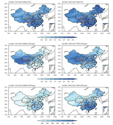
Fig. 1. Multiyear (2001–2019) averaged distributions of diagnosed cloud fields (right) and CERES retrieved cloud products (left). (a, b) Total cloud cover (TCC), (c, d) cloud top height (CTH; km), and (e, f) cloud water path (CWP; μm, equivalent to g m-2).
Whether the diagnostic 3D cloud fields are reasonable and close to the observations is the basis and key difficulty of the CWR-DQ method and its results. Using the monthly averaged total cloud cover (TCC) and CWP products of CERES_SYN1deg_Ed4.1 (https://ceres-tool.larc.nasa.gov/ord-tool/jsp/SYN1degEd41Selection.jsp)from 2001 to 2009, Cai et al. (2020) validated the diagnosed TCC andMhin China and showed that the spatial distributions of the diagnosed TCC andMhwere relatively consistent with the CERES products.
Furthermore, the diagnosed 3D cloud fields are validated with CERES by comparing an extra variable, the cloud top height (CTH; km), in a longer period of 2001–2019 (Fig. 1). In general, the annual average distributions of the diagnosed TCC,Mh, and CTH are consistent with the products retrieved from the CERES satellite observations. The high values of TCC are mainly located over the Sichuan Basin, the Tianshan Mountains,and the Himalayas, while the low values of TCC over the desert areas in Xinjiang, the southern Tibetan Plateau,the Inner Mongolia, and North China. The high values of CERES-CTH are mainly located in the Tibetan Plateau and its southern region, while the low values in the northeastern and southern China. The high-value center of the diagnosed CTH slightly deviates from CERES observation, but the low-value center is consistent. Both the diagnosed and observed CWP gradually decrease from south to north. The high values are located over the Sichuan Basin and the southeast of Zhejiang, Jiangxi,and Hunan, while low values are largely located in the western Xinjiang, Qinghai, Tibetan Region, and some other places of Northwest China (except for the western Tianshan Mountains in Xinjiang). The detailed comparison shows that the diagnostic value is higher than that retrieved from the CERES. Cai et al. (2020) have analyzed the reason and considered that it may be due to the underestimation of TCC and CWP in CERES (Sun-Mack et al., 2007; Xi et al., 2014; Tian et al., 2018).
In general, the diagnostic 3D cloud field products have good consistency with satellite observations. It is preliminarily believed that the results are reasonable and can be used for the diagnostic calculation of CWR.
2.3 Weather modification regions of China and boundary processing method
In the National Weather Modification Development Program released in 2014, according to weather modification operation requirements and plans in China, considering the distribution characteristics of the weather systems, China is divided into six weather modification regions: northeast region, northwest region, north region,central region, southwest region, and southeast region(Fig. 2). In this study, we will focus on the characteristics of CWR in different weather modification regions.
The CWR is quantified for a certain area and time period. According to the definition and calculation formulas of CWR and its related quantities, it can be seen that most variables have different integral dimensions and cannot be simply accumulated. For any study region,in order to determine the outer boundary, the study region needs to be decomposed into grids. In this study,based on the horizontal spatial resolution of the NCEP reanalysis data, the CWR in China is calculated in the 1°× 1° grids, so the regional gridding process also uses the 1° × 1° grids. For example, in Fig. 3 thexandydirections represent different longitudes (I) and latitudes (J).Multiple grids can be decomposed in any latitude direction. The red dot in the figure represents the center point of the grid obtained after area decomposition, and the blue line is the outer grid boundary of the region. For the whole area, the advection of atmospheric water substances only exists along the boundary, while the advection within the region cancels each other out. Here the gray dashed line in the figure is taken as an example for the specific calculation. After the grid processing, the left and right boundaries of the outmost grids are the west boundary and the east boundary at this latitude, respectively. For each latitude, the west boundary and east boundary can be obtained. Then, the meridional outward boundaries of the region can be determined. The zonal outward boundaries of the region are obtained in the same way. Finally, the grids and the outer boundaries of the study area can be determined, and the accuracy depends on the spatial resolution of the reanalysis data.
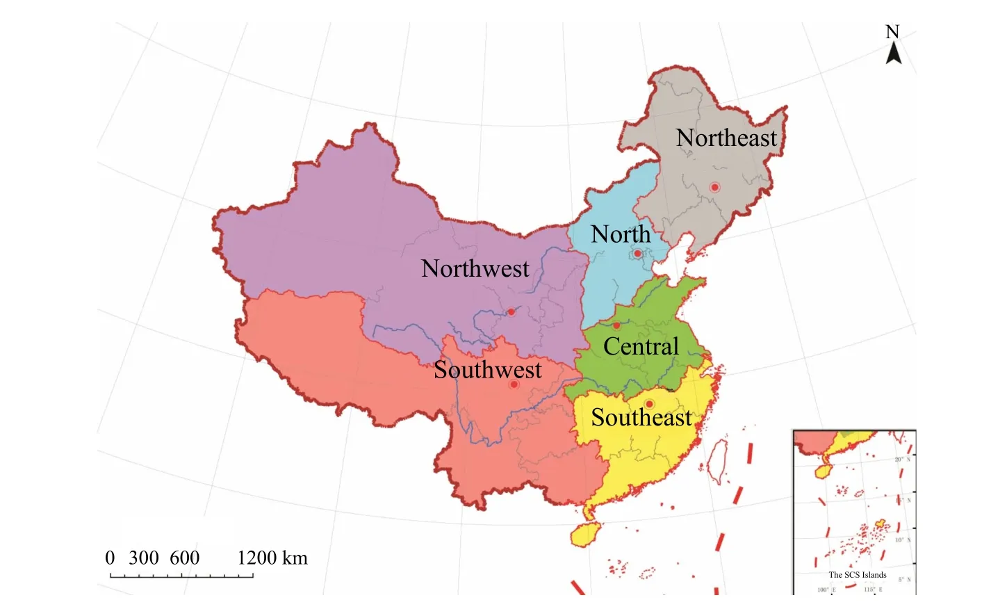
Fig. 2. The weather modification regions in China.
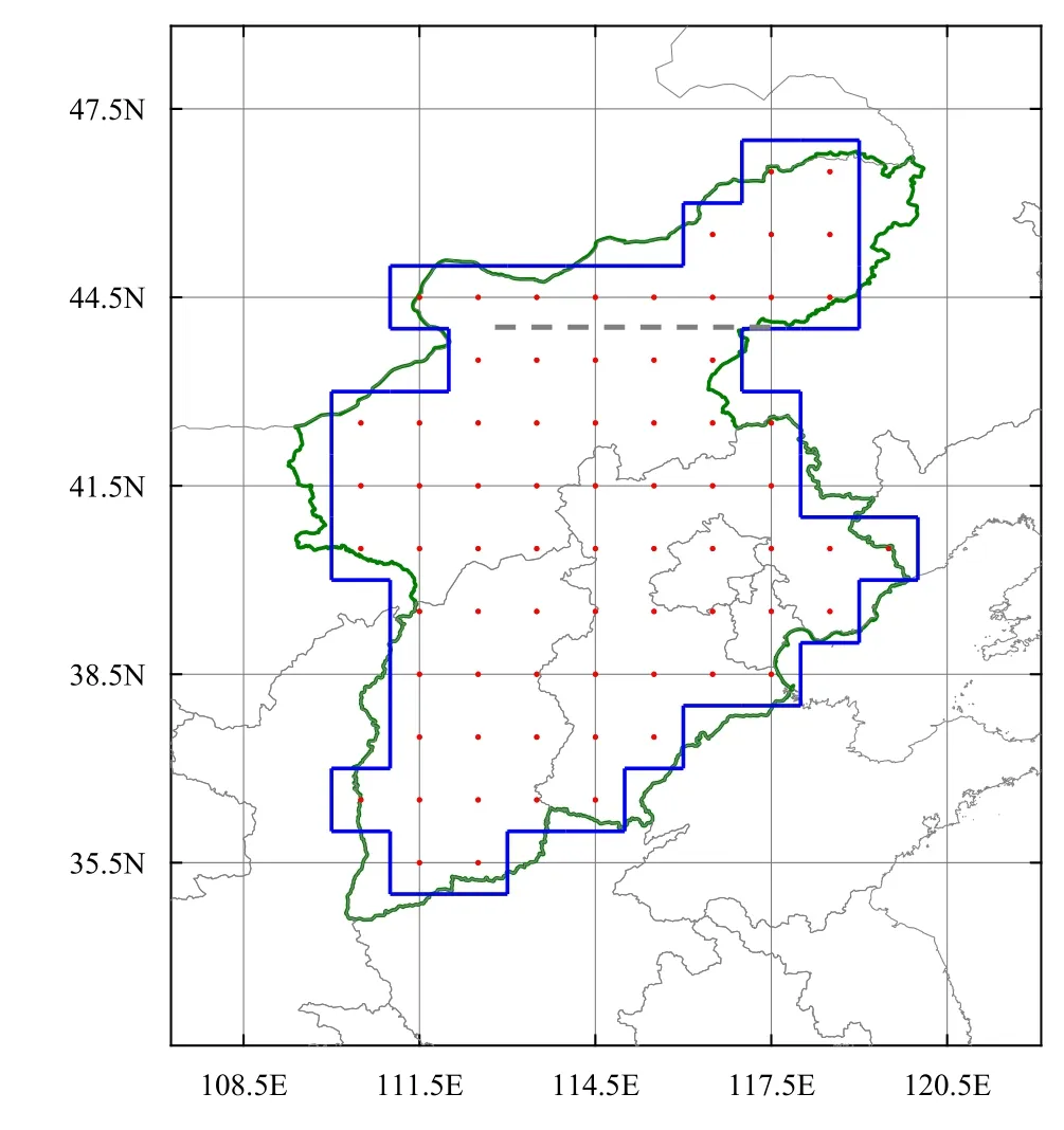
Fig. 3. The schematic diagram of regional gridding and boundary processing. The red dot represents the center point of the grid obtained after domain decomposition. The green line and blue line represent the actual boundary and the processed outer boundary of the region, respectively. For the calculation of regional atmospheric water advection, only those along the blue boundary are counted. The advection inside the study region is not considered because they cancel each other.
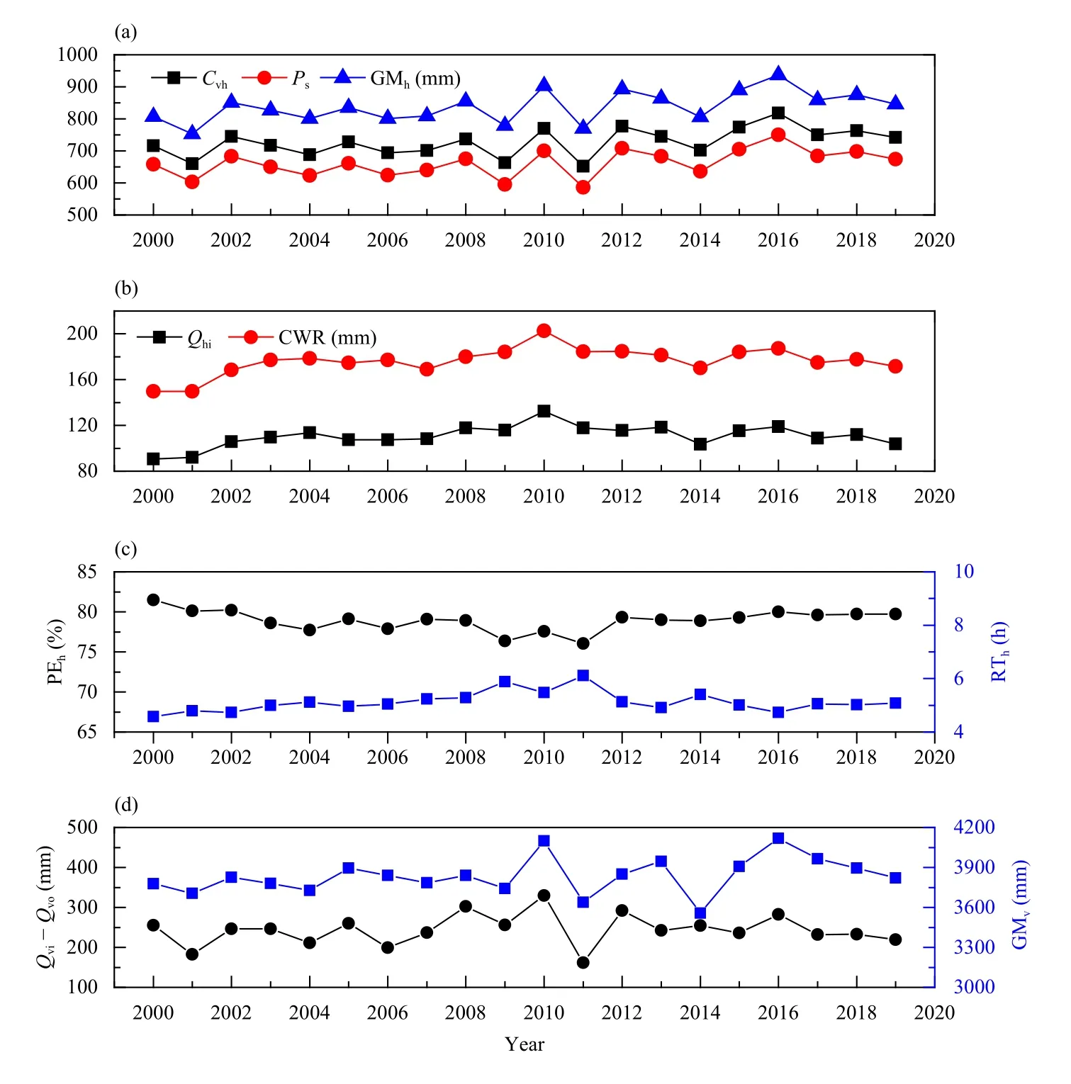
Fig. 4. Annual evolutions of the Chinese CWR and its related quantities from 2000 to 2019. (a) Water vapor converted from hydrometeors through evaporation and sublimation (Cvh), surface precipitation (Ps), and the gross mass of atmospheric hydrometeors (GMh); (b) cloud water resource (CWR) and atmospheric hydrometeors inflow (Qhi); (c) precipitation efficiency and renewal time of hydrometeors (PEh and RTh); and (d)net inflow (Qvi - Qvo) and the gross mass of water vapor (GMv). All the values are annual quantification results. CWR = GMh - Ps, PEh =Ps/GMh.
For CWR quantification in any study area, the principles and methods of spatiotemporal integration are as follows.
(1) Spatial integration. The state variables and sink/source terms are spatially accumulative, while the advection terms are calculated only along the boundaries of the study region.
(2) Temporal integration. With the extension of the calculation period,Mxatt1moment (Mx1) remains unchanged andMxatt2moment (Mx2) becomesMxat the end of the period. The rest 10 quantities (i.e., the advection terms and sink/source terms) can be accumulated over time.
Through the boundary processing method, the deviations between the processed area of the Chinese mainland and six weather modification sub-regions and their actual area are within the range of -2.32% to 4.04%, indicating that the boundary processing method adopted in this study is relatively reasonable.
Furthermore, using the 1° × 1° gridded CWR results of China from 2000 to 2019 and the boundary processing method, we calculate the CWR in the Chinese mainland and the weather modification sub-regions in the past 20 years. Then, the monthly and annual values and the multiyear averaged results are presented, and the characteristics of CWR in different regions are analyzed as follows.
3. Characteristics of CWR in China
3.1 Multiyear average annual results
From 2000 to 2019, the multiyear average of total annualPsin the Chinese mainland was about 6.24 trillion tons (equivalent to about 661.7 mm of column water per unit area). The gross mass of water vapor (GMv) includes the initial water vapor mass (Mv1), the annual water vapor inflow (Qvi), the surface evaporation (Es), and the evaporation from hydrometeors to water vapor (Chv).The calculation formula is GMv=Mv1+Qvi+Es+Chv.The annual GMvparticipated in the atmospheric water cycle in the Chinese mainland was about 36.2 trillion tons on average (about 3835.9 mm). Specifically, the annual average ofMvin the atmosphere (MMv, usually called atmospheric precipitable water before) was about 140 billion tons (approximately 15 mm). The multiyear averages of annualQviandQvowere about 31.6 trillion tons (3347.3 mm) and 29.3 trillion tons (3103.5 mm), respectively. Therefore, the annual convergence (Qvi-Qvo) was about 2.3 trillion tons (243.8 mm). The water vapor had a renewal time (RTv) of about 8 days, and its precipitation efficiency (PEv) was about 17.2%.
Liu and Zhou (1985) calculated the transportation of water vapor in China by using the sounding observation data, and found that the annual total net inflow of water vapor in China was about 2.38 trillion tons. The RTvpresented in Encyclopedia of China was about 8 days(China Encyclopedia General Committee, 1987). According to Gao and Lu (1988), the average annual rainfall in the Chinese mainland was about 700 mm, and the annual evaporation and runoff were about 450 and 250 mm, respectively. In our study,Esis the remainder of the atmospheric water balance equation. The estimated annualEswas 3.97 trillion tons (about 420.5 mm), the annualPswas about 661.7 mm, and thus the annual runoff was about 241.2 mm. The results of water vapor-related quantities and surface water balance calculated by the CWR-DQ method in this paper are generally consistent with previous studies, indicating that the above quantitative results are generally reasonable.
The gross mass of hydrometeors (GMh) is the sum of the initial hydrometeor mass (Mh1), the annual hydrometeor inflow (Qhi), and the condensation from water vapor to hydrometeors (Cvh). The calculation formula is GMh=Mh1+Qhi+Cvh. The annual GMhin the Chinese mainland was about 7.91 trillion tons on average (838.1 mm).Specifically, MMh(similar to CWP termed by previous studies) was about 3.84 billion tons (0.4 mm), less than 3% of MMv. The variablesQhiandQhowere about 1.04 trillion tons (110.8 mm) and 1.07 trillion tons (113.4 mm), respectively. Thus, the annual net inflow of hydrometeors (Qhi-Qho) was about -24.9 billion tons (-2.6 mm). The multiyear average of the annualCvhwas about 6.86 trillion tons (727.1 mm), which was about 10%higher than the annualPs. Besides, the renewal time of hydrometeors (RTh) was about 5 h, and the precipitation efficiency of hydrometers (PEh) was 78.9%. Due to the lack of direct observations of hydrometeor-related quantities and CWR, long-term quantification of hydrometeorrelated variables have not been carried out before, so the verification of the above results is very difficult.However, in Section 2.2 of this study, the diagnostic results of the 3D cloud field distribution in multiple years have been compared with the CERES satellite data. The results show that in general the diagnosed 3D cloud fields are reasonable.
By comparing the results of water vapor-related quantities with hydrometeor-related quantities, it can be seen that in the atmospheric water cycle in the Chinese mainland, there are significant differences between hydrometeors and water vapor. The state quantities, the advection terms, and the gross mass of hydrometeors are smaller than those of water vapor. Different from water vapor,the multiyear averaged annual convergence of hydrometeors is negative. However, RThis short, significantly shorter than RTv, and PEhis much higher than PEv. After deductingPs, the multiyear averaged annual CWR is about 1.66 trillion tons (176.4 mm). Such abundant CWR and rapid hydrometeor renewal are conducive to the atmospheric water cycle and the regeneration and development of CWR in China.
It should be noted that GMhand CWR are discussed for a certain area and period. In previous studies, CWP is an instantaneous quantity that can be observed at a specific moment. It is only a small part of GMhand CWR.The renewal and supplement of hydrometeors should also be considered. Therefore, GMhis a more reasonable quantity than CWP to quantify the total amount of hydrometeors that participate in the atmospheric water cycle in a certain period. The variable GMhreflects the maximum potential of atmospheric hydrometeors that can be converted into surface precipitation, while CWR is the theoretical maximum value of hydrometeors remaining in the atmosphere that can be developed by the technique of artificially precipitation enhancement (APE). Similarly,GMvis also significantly different from the atmospheric precipitable water in previous studies, and the latter is much smaller than the annual GMvandPs.
3.2 Interannual evolution
Figure 4 presents the interannual evolution of CWR and its related quantities in the Chinese mainland from 2000 to 2019. According to the calculation formula of GMh, Zhou et al. (2020) pointed out that when the study period exceeds a month, the contribution ofMhto GMhwill be less than 1%. For the quantification of CWR in large areas,Cvhhas the highest contribution to GMh. In addition, the correlation betweenCvhandPsis the best with a correlation coefficient of more than 0.99. Therefore, the interannual variation characteristics of GMh,Cvh, andPsare very consistent.
According to the definition and calculation formula of CWR (CWR = GMh-Ps), when GMhis large andPsis small, PEhwill be low, and CWR remaining in the atmosphere will be relatively abundant. If GMhis large andPsis relatively abundant, PEhwill be high and CWR will be less. In general, since 2000, CWR in the Chinese mainland has shown a trend of slow increase and fluctuated between 150 and 200 mm, with the least in 2001 (149.6 mm) and the most abundant in 2010 (202.8 mm). A detailed analysis of the various components of CWR shows that the total annualCvhwas the highest (between 660 and 820 mm); the annualPswas slightly smaller thanCvh(about 585–750 mm); and the annualQhitransported from the boundary of the Chinese mainland was significantly less thanCvhandPs(between 90 and 130 mm). ThePsin 2010, 2012, and 2016 was very abundant, of which 2016 was the largest in the past 20 years (750 mm). The variablePsin 2011 and 2009 was less than 600 mm, and the value in 2011 was the lowest in the past 20 years. The results are relatively consistent with the interannual variations of the precipitation observed by national raingauge stations in the past 20 years, which are presented by the “2020 China Climate Bulletin” (CMA, 2021). The variableCvhis also high and low in the more-rain years and less-rain years, respectively.
From 2000 to 2019, PEhgenerally decreased first and then slowly increased, with the value ranging from 75%to 82%; RThgenerally shows a trend of first increasing and then slowly decreasing, with values between 4.6 and 6 h. The inflection points of the interannual variations of the two variables both appeared in 2011, when PEhwas the lowest and RThwas the longest.
Further analysis of the interannual variation of GMvand water vapor convergence (i.e.,Qvi-Qvo) in the Chinese mainland (Fig. 4d) shows that there is a good agreement between the annual water vapor convergence andPs, with a correlation coefficient of 0.63. In the past 20 years, the water vapor convergence in 2011 was the lowest, followed by 2001. In these two years, the annual precipitation in the Chinese mainland was also unusually low. The water vapor convergence in 2010 was the highest, followed by 2008, 2012, and 2016. In these years, the annual precipitation was relatively high. The interannual variations of GMvwere slight in previous years, and became obvious after 2010; GMvin 2010 and 2016 was very abundant, but relatively small in 2011 and 2014.
3.3 Monthly evolution
Figure 5 shows the monthly evolution of CWR related components and characteristic variables in the Chinese mainland from 2000 to 2019. In general, all the variables have obvious seasonal characteristics. Two groups of CWR-related quantities, i.e., CWR andQhi,CvhandPs, have same evolution trends, while PEhand RThhave an opposite trend. The largest values of monthly GMh,Cvh, andPsappear in summer (from June to August), followed by spring and autumn (from March to May and from September to November), and the smallest values in winter (December to February of the next year). From January the three quantities begin to increase, reaching the peak in July (GMh,Cvh, andPswere 139.6, 128.2, and 122.6 mm, respectively), and then decrease until December.
Combining Fig. 4a with Fig. 4c, we find that the monthly variation of PEhis consistent with that of GMhandPs; PEhincreases from January and reaches the peak in July, and then decreases. The monthly variation of RThis the opposite, which gradually decreases from January month by month (i.e., the renewal speed of atmospheric hydrometeor begins to accelerate), reaches the bottom in July, and then gradually increases. It means that in summer, atmospheric hydrometeors renew the fastest and the precipitation efficiency is the highest; while in winter, atmospheric hydrometeors renew the slowest and the precipitation efficiency is the lowest. Consequently, the most abundant GMhin July cannot lead to the highest CWR. According to Fig. 4b, CWR in the Chinese mainland increases from February each year, reaches the annual peak (18.2 mm) in May, and then decreases gradually. Therefore, CWR is abundant in spring and summer(from March to August), followed by autumn and the least in winter. When there is more CWR in the atmosphere, the advection of hydrometeors will be correspondingly stronger. Therefore, the monthly variation ofQhiis more consistent with that of CWR.
The monthly variations of the standard deviations of the CWR related components and characteristic quantities in the Chinese mainland in the past 20 years are shown in Fig. 6. The standard deviations ofCvh,Ps, and GMhhave the same monthly variation trend, with the largest value in summer (July and August, 11.4–11.9 mm),followed by May (9.7–11.2 mm), and the smallest value in winter (from December to the next February, 4.5–6.9 mm). The 20-yr averages of the above three variables are also the largest in summer (74.4–141.0 mm) and relatively smaller in winter (13.3–30.5 mm). Therefore, the relative value of their annual standard deviation (standard deviation/average) is the smallest in summer and the largest in winter (about 10% and 30%, respectively).
The standard deviations of monthly CWR andQhivary slightly, with the largest values in May (2.1 and 1.6 mm,respectively), and the smallest values in July (1.2 and 0.9 mm, respectively). The monthly variations of their 20-yr averages are not obvious, with the smallest from January to February, and the largest in May. Therefore, their relative values of the standard deviation are the largest in January and February (11.5%–15.8%), and the smallest in July when the relative values of the standard deviation of CWR andQhiare only 8.5% and 7.2%, respectively.Moreover, the 20-yr averages of monthly CWR are more than twice of those ofQhi(as shown in Fig. 5), and the standard deviation of CWR is about 60% larger than that ofQhi, leading to a smaller relative value of the standard deviation of CWR than that ofQhi.

Fig. 5. Multiyear (2000–2019) averaged monthly evolutions of the Chinese CWR and its related quantities. Variables in (a), (b), and (c) are the same as Fig. 4. All the values are multiyear averaged monthly results.

Fig. 6. Monthly variations of the multiyear (2000–2019) averaged standard deviation of the Chinese CWR and its related quantities. The quantities are the same as Fig. 5.
The standard deviation of PEhis large in winter(5.7%–10.6%) and small in summer (1.1%–1.6%). Since its average value is small in winter (48.9%–57%) and large in summer (86.4%–87.8%), the relative standard deviation has a much larger value in winter than in summer. The standard deviation of RThis also large in winter(2.4–6.5 h) and small in summer (0.3–0.5 h). Meanwhile,the relative value of its standard deviation is also the largest in winter and smallest in summer. Especially, the value in January reaches 46%, while is only 9.8% in August.
4. CWR characteristics in different regions
The distribution of CWR is very important to the layout planning of weather modification in China. Based on the reasonable results of China’s CWR, the characteristics of CWR in different weather modification sub-regions are further investigated in this study. The multiyear average values of the annual quantification results of CWR and its related quantities in various regions in the past 20 years are listed in Tables 1 and 2, respectively. In order to remove the influence of the study area on the results, CWR and its components, as well as GMxare converted into the value per unit area (kg m-2, equivalent to mm) for comparison and analysis.
4.1 Multiyear averages
4.1.1CWR, GMh, and GMv
According to Table 1, in the past 20 years, GMhper unit area in each region can be sorted from high to low as follows: southeast region (2178.7 mm), central region(1464.4 mm), southwest region (1124.6 mm), northeast region (942.3 mm), north region (830.7 mm), and northwest region (445.1 mm). The variable GMhin the southeast region is almost five times of that in the northwest region. The regional characteristics of annualPsare consistent with GMh, being the most in the southeast region(1640.7 mm), followed by the central region (992.4 mm),the southwest region (877.4 mm), the northeast region(592.4 mm), and the north region (441.8 mm). The annualPsis the least in the northwest region (254.8 mm). After deductingPs, the annual CWR remaining in the atmo-sphere can be sorted from high to low as follows: southeast region (538.1 mm), central region (472.0 mm), north region (388.8 mm), northeast region (350.0 mm), southwest region (247.2 mm), and northwest region (190.3 mm). In other words, CWR is more in the south and the east, less in the north and the west. The variable GMvin each region is generally one order of magnitude higher than GMh, and it can be sorted from highest to lowest as:southeast, central, north, northeast, southwest, and northwest regions. Its regional distribution is different from that of GMhbut is consistent with that of CWR.
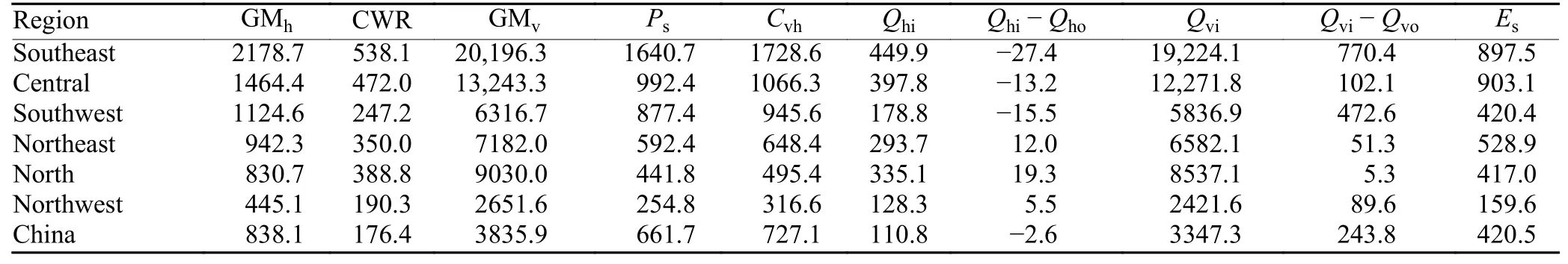
Table 1. Multiyear (2000–2019) averaged values of the CWR, GMh, GMv, and other quantities in the six weather modification regions in the Chinese mainland (kg m-2, equivalent to mm water depth per unit area)
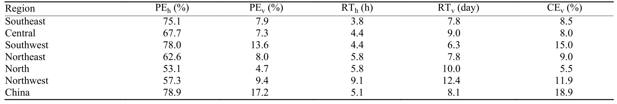
Table 2. Multiyear (2000–2019) averaged value of the conversion efficiency and renewal time of water vapor and hydrometeors in the atmosphere in the six weather modification regions of China. The variables PEh and PEv refer to the precipitation efficiency of hydrometeors and water vapor, respectively (%); RTh and RTv refer to the renewal time of hydrometeors and water vapor with the unit of hour and day, respectively;and CEv refers to the condensation efficiency of water vapor (%)
4.1.2CWR related components
From the comparison of GMhand CWR in Table 1, it can be seen that on average over many years,Cvhin each region contributes the most to GMhand CWR in the region, and is slighter higher thanPsin the region. The order among different regions is consistent with the annualPs, i.e., the highest in the southeast region (1728.6 mm),followed by the central region (1066.3 mm), the southwest region (945.6 mm), the northeast region (648.4 mm),and the north region (495.4 mm), and the least in the northwest region, only 316.6 mm.
The regional deviation ofQhiis smaller than that ofCvh. The variableQhiis still the highest in the southeast region and the lowest in the northwest region. The annualQhiin the other four regions can be listed from high to low as: the central, north, northeast, and southwest regions. The rank ofQviin each region is consistent withQhi, butQviis generally higher thanQhiby a few dozen times. The water vapor advection in each region is expressed as a net inflow (that is, water vapor convergence), and the order from high to low is: southeast, southwest, central, northwest, northeast, and north regions, with the value in the southeast region 127 times of that in the north region. Atmospheric hydrometeor advection in the six regions is different. Hydrometeors in the north, northeast, and northwest regions all show regional convergence (i.e.,Qhi>Qho), while those in the central, southwest, and southeast regions show regional divergence (i.e.,Qhi Detailed analysis shows that there is a good correlation between the annual water vapor convergence and the annualPsin the same region with the correlation coefficient reaching 0.85. In other words, the more water-vapor convergence, the higherCvh, which in turn triggers morePs, such as in the southeast and southwest regions. In addition, Table 1 also presents the results ofEs.Among the six regions, the central region has the largestEs, with an annual mean value of 903.1 mm. The annualEsin the southeast region is about 897.5 mm, only second to that in the central region, followed by the northeast region (528.9 mm), southwest region (420.4 mm), north region (417.0 mm), and northwest region(159.6 mm). Combined with the annualPs, it can be seen that the annualPsis significantly higher thanEsin the southeast, southwest, and northwest regions, andPsin the central, northeast, and north regions is slightly higher than the regionalEs. In general, for regional CWR quantification,Cvhmakes the largest contribution to GMhand CWR. As for the 1°× 1° gridded CWR quantification in North China presented by Cai et al. (2020), the contribution ofQhito GMhand CWR is more important. The reason is that advection cancels each other out within a large area, and only the advection on the boundary is counted, so the effect of the advection terms is weakened (see Section 5.1 for details). Therefore, for atmospheric hydrometeors, the contribution of advection and source/sink terms to GMhis affected by the spatial scale, and there are obvious differences between different spatial scales. However, no matter the quantification is based on 1° interval grids or the overall region, the contribution ofQvito GMvis the highest,which is different from atmospheric hydrometeors. 4.1.3PE, CEv, and RT According to Table 2, the multiyear average values of annual PEhin the six regions are ordered as follows:southwest region (78.0%), southeast region (75.1%),central region (67.7%), northeast region (62.6%), northwest region (57.3%), and north region (53.1%). For RTh,the order from short to long is: southeast region (3.8 h),central and southwest regions (4.4 h), north and northeast regions (5.8 h), and northwest region (9.1 h). Besides, PEvin each region is smaller than PEh, and RTvlonger than RTh. The rankings of PEvand RTvfor different regions are slightly different from those of PEhand RTh, but in general, PE is high and RT is short in the southeast and southwest regions, while low and slow in north and northwest regions. The condensation from water vapor to hydrometeors is mainly affected by terrain uplift and local water vapor content. Therefore, the southwest region with complex terrain has the highest CEv(about 15.0%), followed by northwest region (11.9%), northeast region (8.9%),southeast region (8.5%), and central region (8.0%). The north region has main plains and therefore has the lowest CEvof only 5.5%. Among the six regions, the southeast region has a relatively large GMh. Although the clouds in the southeast region have a higher precipitation efficiency, there are still a large part of the hydrometeors remaining in the air which can be developed and utilized by artificial weather modification. Therefore, CWR in the southeast region is also the most abundant. In the northwest and north regions, GMhis relatively small but PEhis low, so there is still a certain amount of CWR available for development and utilization. Figure 7 presents the interannual variation of CWR and its related quantities in the six sub-regions from 2000 to 2019. The CWR-related quantities in various regions in the past 20 years have shown a fluctuation trend. Specifically, two groups of quantities, i.e., annualPsandCvh,annualQhiand CWR, show similar interannual variation characteristics. The interannual variation ofPsin the southeast region(Fig. 7a) is very dramatic. The variablePsin the wet year(2016, with an annualPsof 2157.8 mm) was almost double that in the dry year (2011, 1247.5 mm). The variable PEhwas the lowest in 2011 (68.7%). In other years,PEhgenerally exceeded 70%. In the southwest region(Fig. 7b), the interannual variation ofPswas not obvious,butPsand PEhdecreased slightly in the past 20 years. In 2009,Psand PEhwere only 748.3 mm and 74.8%, respectively. In the central, north, northeast, and northwest regions (Figs. 7c–f), the lowest values ofPsall occurred in 2001. Specifically,Psin the northwest region showed an increase trend. The variable PEhof the above four regions in the past 20 years generally fluctuated. Among them, PEhin north and northwest regions kept stable during 2000–2010 and increased after 2010. The variable PEhcontinuously increased since 2001 in the northeast region. In the central region, PEhdecreased slightly before 2011, but there were multiple peaks in the past 10 years. Fig. 7. Interannual variations of CWR and its related quantities in the six weather modification regions in China from 2000 to 2019. (a–f) represent the southeast, southwest, central, north, northeast, and northwest regions, respectively. All the values are annual results. Fig. 9. Multiyear (2000–2019) averaged monthly variations of (a) PEh (%) and (b) RTh (h) of the six weather modification regions in China. All the values are multiyear averaged monthly results. In the southeast, southwest, north, and northwest regions, CWR andQhiincreased in volatility since 2000,reached a peak value in 2010, and then decreased in volatility. CWR andQhiin the central region showed a quasi-7-yr periodic variation, while the interannual variations of CWR andQhiin the northeast region were the most obvious. Using the observation data from the national meteorological stations from 1956 to 2013, Ren et al. (2015) analyzed the variation trend of precipitation in China, and they pointed out that the decrease of annual precipitation mainly occurred in North China and Southwest China,while the annual precipitation increased obviously in Northwest China and other regions. Their results are quite consistent with our conclusions. Figures 8 and 9 show the monthly variations of CWR related components and characteristic quantities in the six sub-regions from 2000 to 2019. (1) CWR and its components The monthlyCvhin each region is generally slightly higher than the regionalPs, and the trends of the two are similar. In the monthly variation curves ofCvhandPsin the southeast region, there are multiple peaks, and the main peak appears in June (CvhandPsare 292.7 and 285.4 mm, respectively) with other small peaks in August and November.CvhandPsin the other five regions all present a single peak distribution, with the peak ofPsin July. In general,Psis higher in the central region, and is lower in the northwest region. The monthlyQhiin different regions is generally less thanCvhandPsin the same month. The monthly variations ofQhihave obvious seasonal characteristics. In the southwest, northeast, north, and central regions,Qhiis the highest in summer, followed by spring and autumn, and the least in winter. In the southeast and northwest regions,Qhiis the highest in spring. In the southeast region,Qhiin the first half of the year is significantly higher than in the second half, and the monthly meanQhiis the highest among the six regions. In the other five regions,the monthly variation ofQhiin spring and autumn is relatively small. The variableQhiin each month in the central region is generally higher, followed by the north,northeast, southwest, and northwest regions. Affected by the monthly variations ofCvh, GMhin the southeast region has a multipeak distribution throughout the year, with the highest peak in June (close to 350 mm)and small peaks in August and November. In July, GMhin the southeast region is slightly lower than that in the central region, while in other months GMhin the southeast region is generally higher than that in other regions.Except for the southeast region, the monthly variations of GMhin other regions present a single-peak distribution.That is, GMhbegins to increase from January, reaches the peak value in July, and then decreases gradually. The monthly GMhof the central region is higher than that of other regions in the same month, and the monthly variation and deviation are more obvious (50–250 mm). The monthly GMhin the northwest region is the lowest, and the monthly variation is relatively small (20–60 mm). The monthly variation curve of CWR is relatively similar to that ofQhi. CWR in winter is the least throughout the year in the six regions. In the southeast and northwest regions, the most abundant CWR is in spring, while in the other four regions CWR is more abundant in summer. In the southwest region, CWR in summer is significantly higher than that in autumn by about 30%. In other regions, the CWR in spring and autumn is close to that in summer, with the deviation ranging from 0.6% to 21%. (2) PEhand RTh In the past 20 years, the monthly variation of PEhin six regions is consistent with that of precipitation. The highest PEhis in summer (65%–88%), followed by autumn (25%–82%) and spring (20%–78%), and the lowest value is in winter (14%–65%). Except the southeast region, PEhin other five regions all reaches their peak in July. The difference of PEhin different months in the northeast and north regions is large, and the seasonal difference is more obvious. In the northeast region, PEhis close to 80% in summer and less than 30% in winter; in the north region, PEhcan reach 70% in July but less than 15% in December. In the southeast region, PEhexceeds 80% in summer, and the values in June and August are slightly higher than in July. The monthly variation of RThis opposite to that of PEh, with the shortest RThin summer and the longest RThin winter. In the southeast, southwest, and central regions, the monthly variation of RThis relatively small. In these regions, RThis only about 3 h in summer and less than 15 h in winter. In the northeast, northwest, and north regions, the seasonal differences of RThare quite obvious. Taking the north region as an example, RThis 3–4 h in summer and dozens of hours in winter. RThis closely related toMhand monthly precipitation in different regions and different months. Since precipitation in each region is the highest in summer and the lowest in winter throughout the year, it can be inferred thatMhin each region is also the largest in summer and the least in winter. Comparing the CWR characteristics of six regions in our study with the results of Zhou et al. (2020) on the 1°× 1° grids in North China, we can see the influence of spatial scale on the quantified results. For the 1° × 1° grid study,Qhi(the advection term) makes the highest contribution to GMhand CWR, followed byCvh(the source term), and the contribution ofMh(the state quantity) is the smallest. For large-region quantification, the contribution ofMhis still the smallest, but the contribution ofCvhto GMhand CWR increases, far exceeding the advection terms. The reason is that the quantification of CWR and its related quantities is affected by the spatial scale,especially forQhi. For a large area composed of many grids,Qhicancels each other out within the area, and only the advection along the outer boundary of the area is retained, which is much smaller than the totalQhiof all the grids. However, CWR and other components, such asMh,Ps, andCvh, are the accumulation of all grid values in the area, and they are not affected by the study area.Therefore, as the spatial scale (region area) increases, the advection terms cannot be accumulated, so its importance gradually decreases, while the contributions ofCvhand other source/sink terms gradually increase. However,regardless of the study area, the contribution ofQvito GMvis the highest. Due to the spatial integral characteristics of the advection term, the quantified CWR result in the Chinese mainland is not equal to the sum or average of that in the six weather modification regions. Specifically, the advection terms, GMx, and CWR in the Chinese mainland are less than the sum of the corresponding values in the six regions, and PExand CEvof the Chinese mainland are higher than the corresponding values in the six regions and their average values. However, the convergence of atmospheric water substance (Qxi-Qxo) can be accumulated or averaged with scale. For example, the water vapor convergence (Qvi-Qvo) of China is equal to the sum of that in the six regions. For the result per unit area, it is the average of the six regions, as shown in Tables 1 and 2. It should be pointed out that in the CWR-DQ method,CvhandChvare not directly observed values, but are estimated by the atmospheric hydrometeor balance equation. Cai et al. (2020) compared the diagnosticCvhandChvto their numerical values in two typical months of spring and summer in North China, and the results showed that there is a small difference between the net condensation (Cvh-Chv) obtained by the diagnostic method and its numerical simulation value. The diagnosticCvhandChvare lower than the simulation values, especially in the summer with abundant precipitation when the underestimation ofChvis more obvious. Consequently, GMhand CWR quantified by the diagnosis method might be lower than the actual values, but PEhmight be higher. In the future, it is necessary to further optimize and improve the calculation ofCvh-Chvto improve the diagnosis and quantification accuracy of CWR and its related quantities. In addition, different atmospheric reanalysis data may also have a certain impact on the results. In the future, more atmospheric reanalysis data can be used for the calculation and comparative analysis of CWR quantification. The use of CWR should consider social and economic demands. CWR exists in a short time and limited area.The development of CWR has a positive effect on agricultural drought alleviation, reservoir water storage, ecological restoration, fire extinguishing, and groundwater supplementation, and can make major social and economic benefits. On the contrary, during the flood season or heavy rainfall period, the development of CWR might have negative effects. In different regions of China,the demand for artificial weather modification and the characteristics of local CWR are quite different. The development and utilization of CWR should be comprehensively considered according to the demand and CWR characteristics. North China (the north region in this study), the core area of China’s political culture, faces the demands of ecological protection and agricultural and economic crop production. In this region, the difference betweenPsandEsis only 24.8 mm, which means a very prominent contradiction between water supply and demand. Therefore,it is the region with the most serious water shortage per capita in China. The northwest region has the most concentrated ecological function zones in China. These two regions have the strongest demand for artificial precipitation enhancement and CWR development. According to our study, PEhin the north region and northwest region is not high (53.0% and 57.1%, respectively), and RThin the two regions is short (5.8 and 9.1 h, respectively). Therefore, there is abundant CWR in the atmosphere that can be used by weather modification. In summer, PEhis the highest and the water substance renews the fastest throughout the year; in winter, the case is on the contrary. There are certain limitations in the development of CWR in both summer and winter. In spring and autumn,PEhand RThare moderate. More systematic precipitation processes occur and GMhis also high, leading to a greater potential for the development of CWR through APE. Consequently, in these two regions, spring and autumn are the most suitable seasons for APE, which is consistent with the actual local weather modification operations. The northeast and central regions are the key areas for food production and ecological protection in China. In the two regions, the central region has higher annual precipitation (nearly 1000 mm), only second to the southeast region. In spring, autumn, and winter, PEhis between 40% and 66%, and CWR is abundant, which makes it suitable for APE operations. In the northeast region, the annual precipitation is about 580 mm, and PEhis more than 70% in summer, which is not suitable for APE. In winter, PEhis low, and the temperature of entire atmosphere layer is low with only little supercooled cloud water, which is also not conducive to the artificial operation of cold cloud. Therefore, spring and autumn are more suitable for the CWR development and utilization in the northeast region. The southwest region is an important characteristic agricultural production base and the largest flue-cured tobacco production base in China. The annual precipitation in this region is about 875 mm, with PEhexceeding 70% from April to October. Due to the complex terrain and mountains, convective rainfall and hail are more likely to occur, causing geological disasters and socialeconomic losses. Therefore, for the CWR development in this region, we should pay more attention to the hail prevention through rocket and artillery operation in spring,summer, and autumn, and avoid developing cloud water resources during the heavy rainfall season (summer). The southeast region is the key area for grain production and ecological protection. The surface precipitation in this region is much higher than that in other regions.The difference between the annualPsandEsis 743.2 mm, so the demand for precipitation enhancement and drought resistance is small. Especially in summer, PEhexceeds 80%, and RThis very short (less than 3 h),which is easy to cause flood disasters. In winter, the precipitation is relatively weak, and PEhis also reduced.Therefore, the demand for APE to develop CWR is more concentrated in winter or the transition period from winter to spring. In this study, 3D cloud fields with the resolution of 1°× 1° from 2000 to 2019 in China are firstly obtained from the NCEP reanalysis data. Based on the CWR-DQ method, combined with the GPCP products, a 1° × 1°gridded CWR dataset of China in recent 20 years is established. On this basis, through the processing of region boundaries, the monthly and annual variations of CWR and its related variables are investigated in China and the six weather modification regions. Furthermore, the characteristics of CWR development in different regions are discussed. The main conclusions are as follows. The 3D cloud fields of China during 2000–2019 are diagnosed and compared with CERES products. The results show that the multiyear averaged distributions of TCC, CTH, and CWP obtained by the diagnostic method are consistent with those of CERES observations. In the past 20 years, GMhin the Chinese mainland was about 7.91 trillion tons (equivalent to about 838.1 mm of column water per unit area), and GMvwas about 36.2 trillion tons (3835.9 mm). After deducting the annual precipitation (Ps, 6.24 trillion tons, i.e., 661.7 mm), the annual CWR was about 176.4 mm. PEhand PEvwere about 78.9% and 17.2%, respectively; RThand RTvwere about 5 h and 8 days, respectively. Among the six weather modification regions, the southeast region has the largest amount of cloud condensation (Cvh) and precipitation, leading to the most abundant GMhand CWR in this region, while the annualPs, GMh, and CWR in the northwest region are the least.The annual PEhin the southwest region is the highest(78.0%), and that in the north region is the lowest(53.1%). CEvis affected by terrain uplift and local water vapor content. It is the highest (15.0%) in the southwest region with complex terrain and the lowest (5.5%) in the north region with large plains. The monthly and interannual variation trends ofPs,Cvh, and GMhin different regions are similar, while the variation characteristics of CWR andQhiare consistent.The annualPsand CWR in the Chinese mainland were the least in 2001, and the most abundant in 2010. CWR in the north, northwest, southeast, and southwest regions fluctuated and increased since 2000, reached the peak in 2010, and then decreased in volatility. The interannual variation of CWR in the northeast region is obvious. The CWR in the central region shows a quasi-7-yr periodic variation. In the north, northwest, and northeast regions, PEhis relatively not high (20%–60%), RThis relatively long(5–25 h), and GMhis relatively high in spring and autumn. Therefore, there is greater potential for the development of CWR through the APE. For the central region,spring, autumn, and winter are the more suitable seasons for CWR development. In the southwest region, more attention should be paid to the ground hail prevention in spring, summer, and autumn. For the southeast region,the development of CWR should be concentrated in winter or the transition period from winter to spring. For both regions,Psand PEhin summer are so high that the development of CWR should be avoided in case of floods. The quantifications of CWR and its related quantities are affected by the spatial scale. The advection of hydrometeors makes a greater contribution to GMhand CWR in a small area (such as a 1° grid), while the contribution of condensation is higher for a larger area. In the atmospheric water cycle, there are significant differences between water vapor and hydrometeors. The state quantity and the total amount of atmospheric hydrometeors are much smaller than those of water vapor. Different from water vapor, the annual average advection of hydrometeors in the Chinese mainland is net outflow. However, atmospheric hydrometeors have a shorter renewal time and higher precipitation efficiency. In general, we calculate the CWR and its related variables in China and the six sub-regions, and detailedly analyze the characteristics of CWR in each region. The development and utilization of CWR should be carried out in accordance with local demands and the characteristics of CWR. In the future, it is necessary to strengthen the research on the coupling utilization of CWR, terrestrial water resources, and other various needs. The development of CWR should also be closely combined with terrestrial hydrology and disaster prevention and mitigation. More in-depth research on the characteristics and the change laws of CWR in various regions will be carried out to provide a basis for the planning and layout of local weather modification operation and guidance of the CWR development.4.2 Interannual variation

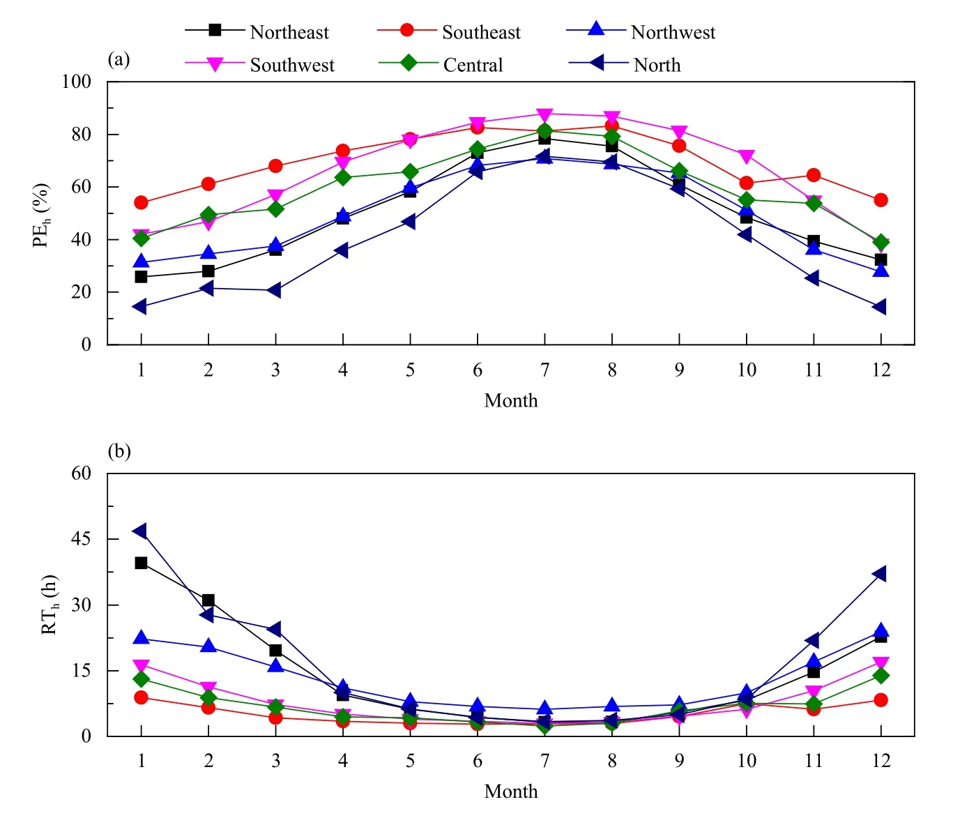
4.3 Monthly variation
5. Discussion
5.1 Influence of spatial scale on the quantified results
5.2 Development and utilization characteristics of CWR in various regions
6. Conclusions
 Journal of Meteorological Research2022年2期
- Journal of Meteorological Research的其它文章
- An Updated Review of Event Attribution Approaches
- CMIP6 Projections of the “Warming–Wetting” Trend in Northwest China and Related Extreme Events Based on Observational Constraints
- Role of Anthropogenic Climate Change in Autumn Drought Trend over China from 1961 to 2014
- Deep Learning for Seasonal Precipitation Prediction over China
- Contribution of Winter SSTA in the Tropical Eastern Pacific to Changes of Tropical Cyclone Precipitation over Southeast China
- Factors Influencing Diurnal Variations of Cloud and Precipitation in the Yushu Area of the Tibetan Plateau