Deep Learning for Seasonal Precipitation Prediction over China

Weixin JIN, Yong LUO*, Tongwen WU, Xiaomeng HUANG, Wei XUE, and Chaoqing YU

1 Department of Earth System Science, Ministry of Education Key Laboratory for Earth System Modeling, Institute for Global Change Studies,Tsinghua University, Beijing 100084

2 Beijing Climate Center, China Meteorological Administration, Beijing 100081

3 AI for Earth Lab, the Joint Laboratory of Cross-Strait Tsinghua Research Institute, Xiamen 361006

ABSTRACT Despite significant progress having been made in recent years, the forecast skill for seasonal precipitation over China remains limited. In this study, a deep-learning-based statistical prediction model for seasonal precipitation over China was developed. The model was trained to learn the distribution of the seasonal precipitation using simultaneous general circulation data. First, it was pre-trained with the hindcasts of several general circulation models(GCMs), and evaluation of the test set suggested that the pre-trained model could basically reproduce the GCM-predicted precipitation, with the anomaly pattern correlation coefficients (PCCs) greater than 0.80. Then, transfer learning was applied by using ECMWF Reanalysis v5 (ERA5) data and gridded precipitation observational data over China, to further correct the systemic errors in the model. As a result, using general circulation fields from reanalysis as the input, this hybrid model performed reasonably well in simulating the seasonal precipitation over China, with the PCC reaching 0.71. In addition, the results using the circulation fields predicted by GCMs as the input were also assessed. In general, the proposed model improves the PCC over China by 0.10–0.13, as compared to the raw GCM outputs, for lead times of 1–4 months. This deep learning model has been used at the National Climate Center of China Meteorological Administration for the past two years to provide guidance for summer precipitation prediction over China and has performed extremely well.

Key words: seasonal precipitation, seasonal prediction, statistical downscaling, deep learning

1. Introduction

The seasonal variability of precipitation has a considerable impact on many sectors, such as agriculture, water resources, economy, transportation, human health,and natural environment. Skillful precipitation forecasts can help in socioeconomic decision-making, such as water management and flood warnings, to reduce the damage caused by weather-related disasters. However, due to the remarkable variability of the East Asian monsoon and complex topographic effects, seasonal precipitation forecasts in China remain a major challenge.

Seasonal precipitation forecast models can be broadly classified as dynamic, statistical, and dynamic–statistical methods. Dynamic models are developed based on the physical laws of the climate. Although seasonal dynamic models have made significant progress over the past few decades, they still do not perform well in the seasonal forecasting of precipitation in the middle to high latitudes (Wang et al., 2009; Luo et al., 2013; Peng et al.,2013; Mishra et al., 2019). The seasonal precipitation forecast skill over land is generally lower than over the tropical oceans (Saha et al., 2014; Johnson et al., 2019).Furthermore, based on summer rainfall hindcasts initiated in May from eight seasonal forecast systems participating in the North American Multi-Model Ensemble,Liang et al. (2019) reported low skill over China with linear correlation coefficients of -0.3 to 0.5 with observations.

Due to the limited forecast skill and high requirement for computational resource and data storage of current operational dynamic models, statistical modeling is still widely used to produce seasonal precipitation forecasts.Statistical methods, such as linear regression (Wang B. et al., 2015; Kämäräinen et al., 2019), usually relate climatic variables from previous months to precipitation empirically, based on historical data. The established relationship is then used for out-of-sample data to make precipitation forecasts. The useful statistical information is extracted from the parameters varying slowly with time and acting as forcing for future seasonal precipitation, such as the sea surface temperature, snow cover, and sea ice. For example, large-scale climate oscillations, such as EI Niño–Southern Oscillation, are good indicators of the seasonal precipitation distribution at low and mid latitudes (Wu et al., 2003; Xiao et al., 2015; Wen et al.,2019).

Dynamic–statistical models take advantages of both physical and empirical methods. There are two aspects to incorporate from physical and empirical models: Model Output Statistics (MOS) and Perfect Prognosis (PP)(Marzban et al., 2006). The MOS technique is aimed at correcting systemic errors by matching the predictands of dynamic models and the same variable of observations.The PP technique constructs statistical relations between the large-scale indicators and local-scale predictands(Klein, 1982). The indicators are generally restricted to the circulation variables that are directly resolved by discretizing the atmospheric dynamics equations with higher forecast skill. A typical predictand is precipitation, which is generated by parameterization schemes in dynamic models (Pan et al., 2019). General circulation models(GCMs) are typically too coarse to represent local features. In this case, the PP technique serves as a downscaling method establishing a statistical link between large and local scales (Wang X. Q. et al., 2015). A great many variations on the original ideas of PP have been proposed to increase the skill of seasonal precipitation forecasting over China. For instance, Chu et al. (2008) and Liu and Fan (2014) used predictors including 500-hPa geopotential height and sea level pressure from GCMs with singular value decomposition to predict seasonal precipitation. Fan et al. (2008) and Chen et al. (2012) established multivariate linear regressions between summer precipitation over China and seven large-scale circulation variables from GCMs that were highly correlated with precipitation. The main disadvantage of the PP technique, however, is that it takes no account of errors in the large-scale circulation forecasts. For this reason, some previous studies have combined simultaneous circulation variables from GCMs with precursors from observations. For example, Dai and Fan (2021) selected six predictors, including predictors from GCMs and observational data, including sea surface temperature in the preceding winter and sea–ice concentration in the preceding winter and autumn over key regions, to predict summer precipitation over China.

Recently, the rapid progress in deep learning has also shown strong potential in seasonal prediction. With the advent of the “big data” era, deep learning has had dramatic impacts in many different fields. At the same time,a deluge of climate data has become available, coming from various observation systems and dynamic models(Reichstein et al., 2019). Deep learning has already made some progress in atmospheric sciences. Examples include deep learning for precipitation nowcasting (Shi et al., 2017; Sønderby et al., 2020; Trebing et al., 2021), the recognition of extreme events (Liu et al., 2016; Racah et al., 2017), postprocessing ensemble weather forecasts(Rasp and Lerch, 2018; Grönquist et al., 2021), and replacing the traditional sub-grid parameterizations in numerical models (Rasp et al., 2018; Gagne et al., 2020).On the seasonal timescale, there is normally not enough observational data to train a deep learning model. Instead, simulated data from numerical models have been used to pre-train the deep learning model, followed by fine-tuning with observations (Ham et al., 2019; Kadow et al., 2020).

Deep learning allows a model to be fed with raw data and for the predictors to be automatically discovered without careful feature extraction and transformation of the raw data, which require considerable subject expertise (LeCun et al., 2015). In particular, convolutional neural networks (CNNs) are designed to process multidimensional arrays—for example, a color image—to recognize the pattern of different spatial scales. In this paper, we introduce a CNN model to serve as a downscaling method to forecast seasonal precipitation over China.The reasons for choosing a CNN are twofold. First,CNNs use nonlinear functions to reveal more complex relationships compared to conventional statistical methods. Second, instead of choosing hand-engineered features from experience as predictors, we can use the raw grid values of general circulation as the input to automatically extract useful and significant predictors from the general circulation for seasonal precipitation forecasts over China, and even to provide valuable insights into the statistical linkages inside the climate system that are revealed.

2. Data and methods

2.1 Data

The hindcast simulations spanning 1994 to 2016 produced by five dynamic global seasonal forecast systems were used to pre-train the deep learning model. Details of the models are given in Table 1. To greatly increase the number of training data, each single ensemble member was used as a data sample. As a result, the total number of samples is 163,392. The grid data were interpolated to the same grid with a resolution of 1° × 1°. The period for training the model was from 1994 to 2008. Data from 2009 to 2012 were used to validate the model. The forecast skill was tested with the data from 2013 to 2016.The validation set was used to calibrate the model hyperparameters and prevent overfitting.

Table 1. Details of the hindcasts

Reanalysis and surface precipitation observations were used to optimize the statistical model. Specifically,monthly reanalysis data from the ECMWF Reanalysis v5(ERA5; Hersbach et al., 2019a, b) spanning 1979 to 2019 were interpolated at a resolution of 1° × 1°, and a dataset of monthly precipitation observations from 1979 to 2019 on a 0.5° × 0.5° grid was obtained from the National Meteorological Information Centre of the China Meteorological Administration (Zhao et al., 2014). This dataset was interpolated from the records of 2474 national-level ground stations using the thin-plate spline method. All these data were converted to a seasonal scale with a three-month moving window from January–February–March to December–January–February.

In order to reduce the dimension of the predictands, an empirical orthogonal function (EOF) analysis of seasonal normalized precipitation observations was performed from 1994 to 2008. Note that the precipitation was nor-malized by each season, while the EOF analysis was performed with normalized precipitation in all seasons. The normalized precipitation in the numerical model hindcasts was projected onto the EOF patterns of the observations to gain a better training effect.

2.2 Methods

2.2.1Convolutional neural network

A deep neural network is a multilayer stack of artificial neural networks that simulate nonlinear input–output mappings. The coefficients in this architecture can be trained by back propagation and gradient descent(Rumelhart et al., 1986). A CNN is a particular type of deep neural network with only local connections between layers. The same coefficients are shared at different locations to reduce the number of coefficients and detect the same pattern in different parts of the array (LeCun et al.,2015).

A typical CNN is composed of convolutional layers and pooling layers. Each convolutional layer is followed by an activation function to introduce nonlinear fitting.The role of the pooling layers is to merge adjacent features and to reduce the size of the model. The hierarchical structure of the convolutional and pooling layers extracts features of different spatial scale by different layers(Zeiler and Fergus, 2014).

Our CNN model used gridded circulation variables over 20°S–70°N, 0–180° as predictors. To be specific,the seasonal anomaly field of zonal wind speed (U) at 200 hPa, geopotential height (Z) at 500 hPa, specific humidity (Q), zonal and meridional wind speed (V) at 500/700/850 hPa, mean sea level pressure (MSLP), and 2-m temperature (T2m) were stacked as a 3D array with 13 channels. The predictand to be downscaled was the principal component (PC) of the simultaneous normalized precipitation anomaly over China.

2.2.2Convolutional block attention module

In addition to the standard CNN, we propose adding an attention mechanism called the convolutional block attention module (CBAM) to every CNN layer (Woo et al., 2018). CBAM multiplies the feature maps of the CNN layers by the weights across channels and spatial dimensions, which are generated by additional lightweight neural networks. CBAM facilitates the network to focus on specific parts of the feature maps (hence the name “attention”).

2.2.3Ridge regression

Ridge regression addresses some of the problems of the ordinary least-squares method in linear regression by imposing a penalty on the size of the coefficients:whereXdenotes the predictors,ydenotes the predictands,wdenotes the coefficients, and the complexity parameterα≥ 0 controls the amount of shrinkage. It is widely used in scenarios where independent variables are highly correlated.

2.2.4Model

The deep learning model proposed here was built upon a CNN and CBAM architecture, as shown in Fig. 1. On account of the samples from different seasons being trained by a single model, an additional season channel embedded from one-hot encoding was concatenated to the input. An activation function called “tanh” was added after every CNN layer. Layer normalization (Ba et al., 2016) was integrated to reduce the training time. We also included the dropout layer (Srivastava et al., 2014)in the fully connected (FC) layer, addressing the problem of overfitting. The mean square error (MSE) was adopted as a loss function. We retained all the EOF patterns but weighted the MSE of each PC by the explained variance ratio to focus on the leading patterns. AdamW(Loshchilov and Hutter, 2019) with weight-decay was chosen for model optimization. The learning rate reduced automatically or early-stopped the training process when the performance based on the validation dataset stopped improving.

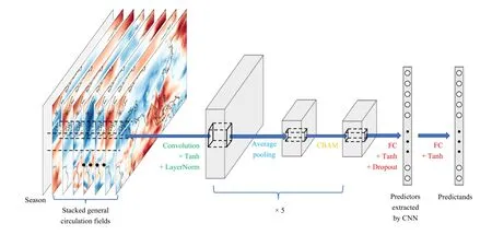
Fig. 1. Architecture of the model used for precipitation downscaling. Five similar modules each consisting of convolution, pooling, and CBAM layers are stacked successively. The last layer is the FC layer, which is trained with numerical hindcasts and modified by ridge regression during transfer learning.

2.2.5Training strategy

The model training was divided into two phases. First,it was pre-trained based on the general circulation and PCs of precipitation in the dynamic model hindcasts. In this phase, the model learned to represent the precipitation-related parameterization schemes in the dynamic models. In the second phase, in consideration of the short period of observational data, the data from the “real world” was utilized by the simpler ridge regression. The coefficients in the pre-trained model were frozen and reanalysis data were fed into it to obtain the feature output by the penultimate layer. We believe that these features are valuable indicators in the general circulation.That is, the ridge model was fitted only between the extracted features and the predictands, to correct the systematic errors of the circulation–precipitation relationship learned from the dynamic models. Specifically, in the second phase, the predictands were set to the bias of the pre-trained model—namely, the difference between the predicted and observed PCs, similar to the residual learning (He et al., 2016). Furthermore, the linear regression coefficients in the ridge model were easy to add to the coefficients in the last FC layer of the pre-trained model. Thereby, the architecture of the final hybrid model remained unchanged after this phase. This hybrid model is a combination of knowledge learned from hindcasts via deep learning and additional information learned from observations via traditional statistical modeling.

3. Results

3.1 Verification of the pre-trained model

The deep learning model was first pre-trained with the general circulation hindcasts and the corresponding PCs of the precipitation hindcasts. The normalized precipitation anomaly was reconstructed from the PC output by the deep learning model. The averaged anomaly pattern correlation coefficients (PCCs) and root-mean-square errors (RMSEs) using the test set from 2013 to 2016 between the dynamic precipitation forecast and the deep learning precipitation forecast are shown in Table 2. The PCCs of the deep learning model in the four seasons are above 0.80, while the RMSEs are under 0.60. In addition,the skill of the deep learning model barely affected by the change in seasons, albeit the skill in summer is slightly higher. Note that the deep learning model was trained with each ensemble member of several dynamic models with different parameterization schemes, which may have enhanced the fitting difficulty. Hence, we conclude that deep learning algorithms are capable of simulating the relationship between circulation and precipitation in dynamic models, even when only some of the variables at specific levels are provided as inputs.

In order to test the optimality of the model input configuration, we carried out several experiments by modifying the spatial region of input variables, their selection,and spatial resolution, and compared the results against those in Table 2. As far as possible, the model architecture was kept the same in these experiments. The experimental design and PCC differences are given in Table 3.As can be seen, the model performance based on hindcasts cannot increase any further by modifying the configuration of the input variables.

Table 2. Average PCCs and RMSEs between the normalized precipitation anomaly predictions of the pre-trained model and the hindcasts during 2013–2016. The input of the pre-trained model was the circulation hindcasts

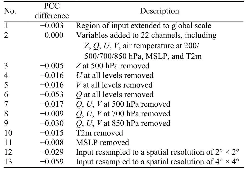
Table 3. PCC difference between different input configurations

In experiments 1 and 2, extending the region of input to the global scale or adding more variables was not helpful for improving the performance, which suggests that the large-scale contextual information is already included in the present input. In experiments 3–11, different variables were removed from the input, and the results demonstrated the need for the current variables and assessed their importance. The PCC in experiment 6 withoutQat all levels decreased by 0.053, which was the most significant compared to other variables in experiments 3–5. This might have been caused by the following two reasons:Qrepresents the moisture transport and is highly correlated to precipitation; andZprovides similar information and can be substituted byUandVwhen it is close to geostrophic flow. Experiments 7–9 further measured the importance of moisture transport at different levels. The PCC decreased by 0.030 withoutQ,U,andVat 850 hPa, which accords with the fact that the moisture was concentrated at this level. Experiments 12 and 13 revealed the effect of the high spatial resolution of the general circulation fields. Reducing the resolution from 1° × 1° to 4° × 4° led to the PCC decreasing by 0.059, which hints at the learning ability of the deep learning model for small-scale circulation variability.

To further estimate the actual performance of the pretrained model, the same variables of the ERA5 reanalysis data were fed into it, and the model outputs were compared with observations over China. Even if the reanalysis and observational data were not used for training, since the hindcasts were correlated with them, the model was still evaluated only in the time range excluding the hindcast training period, to avoid data leakage. The model trained with dynamic data already exhibited considerable skill compared with observations, with PCCs ranging from 0.54 to 0.64 and RMSEs from 0.84 to 0.97(Table 4). The scores in different seasons fluctuated,probably due to the randomness introduced by the limited number of samples (26 yr season-1).

Table 4. Average PCCs and RMSEs between the normalized precipitation anomaly predictions of the pre-trained model and the observations during 1979–1993 and 2009–2019. The input of the pre-trained model was the circulation reanalysis

In fact, the deep learning model can be regarded as an alternative to the physics parameterization schemes in dynamic models, linking the circulation field and precipitation. As such, our results reflect the ability of the dynamic models to simulate precipitation. The four-season-average PCC in the observation was 0.60, which was lower than in the hindcasts (0.81). This gap represents the residual of the precipitation schemes. On the other hand, the seasonal precipitation forecast skill of state-ofthe-art dynamic models over China is far below 0.60(Johnson et al., 2019; Liang et al., 2019), which suggests that the errors of the circulation forecasts in dynamic models severely limit the seasonal precipitation forecast skill. In other words, notwithstanding the relatively high circulation forecast skill, with a more accurate circulation context, there is still great potential to improve the precipitation forecasting ability of dynamic models,with the same precipitation-related parameterization schemes.

The temporal correlation coefficients (TCCs) of different PCs were also examined (solid line in Fig. 2). The leading PCs of precipitation representing large-scale patterns were more predictable, while the later PCs possessed little skill. Since the model is trained with hindcasts but tested with observations, it suggests that dynamic models can accurately capture the main spatial pattern of seasonal precipitation in China, while the subsequent local-scale patterns cannot be expressed well in global dynamic systems. Additionally, the corresponding TCC of experiment 13 in Table 3 using an input spatial resolution of 4° × 4° is shown by the dashed line. The TCC difference between the two datasets of different resolutions (the bars) increases along with the ranking of the EOF patterns. This validates the previous conclusion that a finer input resolution contributes to capturing the small-scale characteristics of the precipitation distribution.

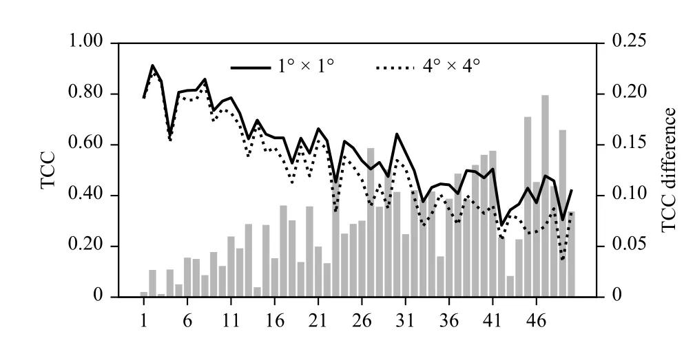
Fig. 2. Temporal correlation coefficients during 1979–1993 and 2009–2019 between the PCs of precipitation observations and the output of the pre-trained model inferred from circulation reanalysis data.The horizontal axis refers to the rank of the PCs. The solid (dashed)line refers to the result with a 1° × 1° (4° × 4°) input resolution. Bars refer to their difference.

Due to the randomness during deep learning model initialization and training, the coefficients will be slightly different each time when the model is trained. To test the impact of this, the model training process was repeated 20 times. The results showed that the standard deviations of the PCCs and RMSEs of each version were smaller than 0.003 and 0.010, respectively, which basically verified most of the conclusions given above, except those for experiments 1–3 in Table 3.

3.2 Verification of the hybrid model

After examining the skill of the deep learning model pre-trained with hindcasts, we subsequently focused on utilizing the reanalysis and observational data to correct the systematic errors of the pre-trained model and improve the seasonal precipitation forecast skill. In the research field of deep learning, models are first trained on a large and general enough dataset. Then, the acquired knowledge can be used for a similar task with a smaller dataset. In this process, called transfer learning, only a few of the top layers of the frozen model are usually“fine-tuned” with the small dataset of the specific problem. However, at present, there is only decades-worth of reanalysis and observational data. As a result, only a few dozen samples are available for model training at the seasonal scale, which is far from enough even for fine-tuning. Therefore, in this study, the reanalysis and observational data were only used for a linear multivariate ridge regression model. This model was superimposed on the last FC layer in the pre-trained model, which is essentially also a linear regression function, as mentioned in Section 2. This hybrid model takes advantage of both the dynamic hindcasts and observational data, as mentioned above.

This model was calibrated and tested by 1-yr-out cross-validation applied to prevent overfitting with data during 1979–2019. Data between 1994 and 2008 were also excluded to avoid data leakage in the evaluation.Figure 3 compares the pre-trained and hybrid model,from which it can be seen that transfer learning clearly improved the ability to simulate precipitation. The fourseason-average PCC increased from 0.60 to 0.71, while the RMSE decreased from 0.90 to 0.72. Moreover, 101 out of 104 test samples exhibited higher PCCs and lower RMSEs in the hybrid model comparing to the pre-trained model. Among the four seasons, the improvement in winter (DJF) was the largest, with the PCC increasing from 0.54 to 0.67.

The TCCs of observed precipitation and downscaling results based on the reanalysis circulation field were also examined. As Fig. 4 demonstrates that, for all four seasons, most of the TCCs (except over a small part of western China) were greater than 0.6, which was far beyond the 99% confidence level. The TCCs over western China were significantly lower than eastern China. In DJF, the TCCs were greater than 0.9 over southeastern China,which indicates that winter precipitation in this region can be inferred very well by the large-scale circulation patterns. By contrast, the TCCs in summer (JJA) and autumn (SON) were distributed more homogeneously over eastern China.

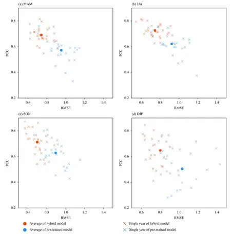
Fig. 3. PCCs and RMSEs of the precipitation anomaly over China in different seasons of the pre-trained and hybrid model during 1979–1993 and 2009–2019. The model inputs were both the circulation reanalysis. The model labels are both the normalized precipitation observations.

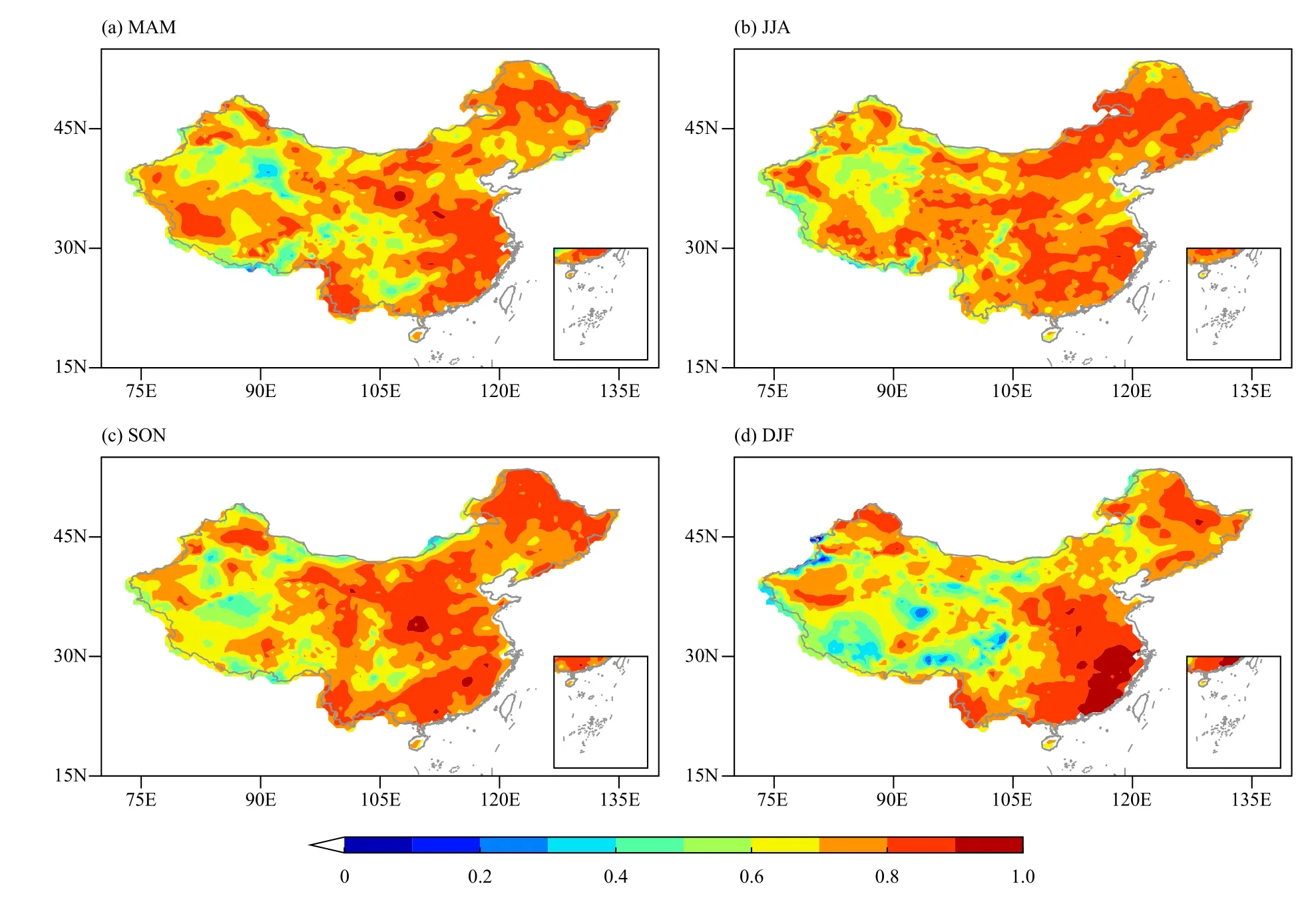
Fig. 4. Spatial patterns of TCCs in different seasons between the observed precipitation and the downscaling results of the hybrid model based on the circulation reanalysis. The evaluation period is 1979–1993 and 2009–2019.

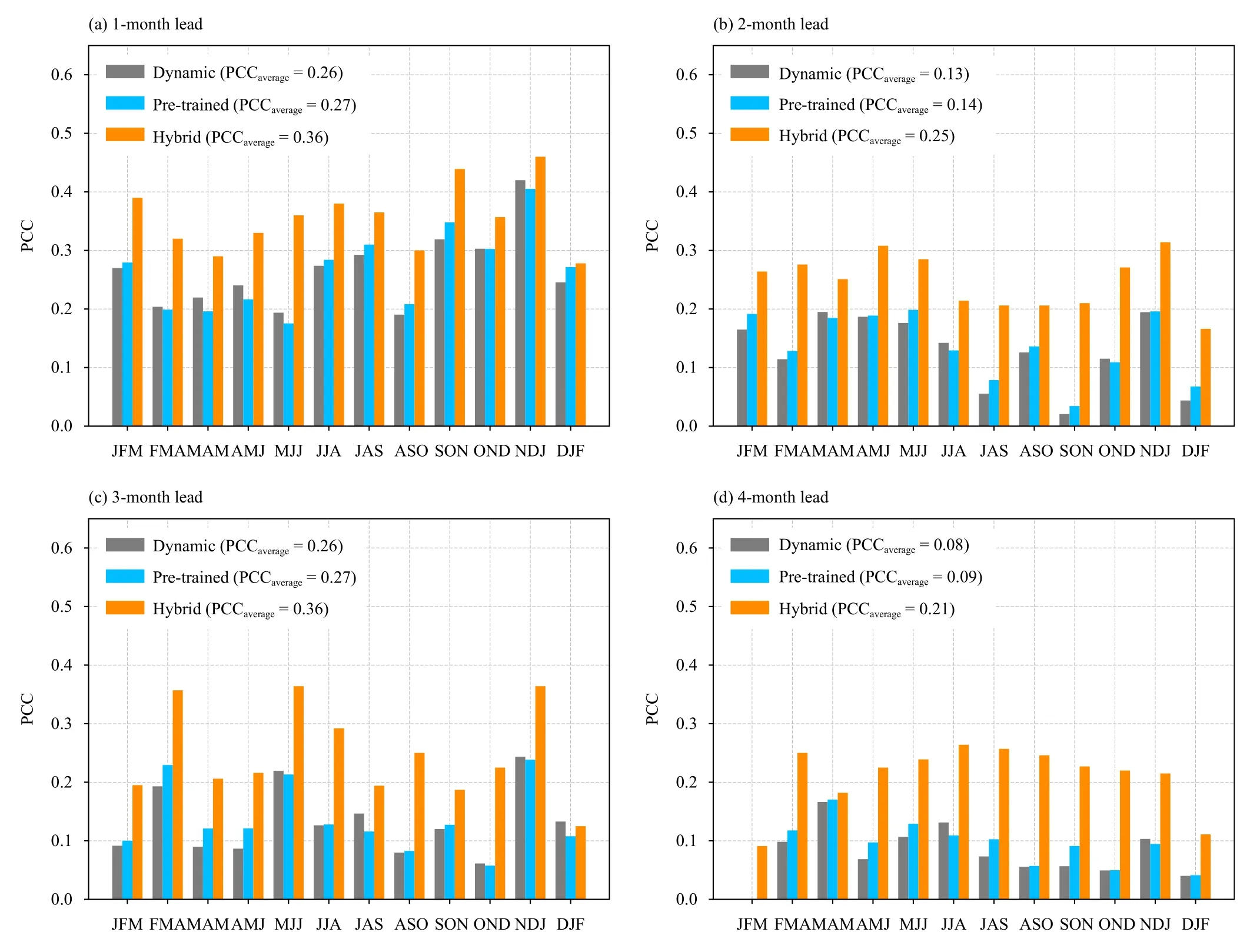
Fig. 5. PCCs of the normalized precipitation anomaly over China in different seasons of the pre-trained, hybrid model, and SEAS5 for different lead times during 2013–2016. For the pre-trained and hybrid model, the input was the circulation hindcasts of SEAS5.

Considering that the input of the ridge regression model was built on the features extracted by this deep learning model, the indication is that deep learning is capable of extracting useful physical factors from large-scale general circulation data for precipitation downscaling. Furthermore, after transfer learning, the performance of the hybrid model with reanalysis and observational data (PCC= 0.71) was close to that of the pre-trained model in the hindcasts (PCC = 0.81), notwithstanding the number of hindcast samples was far more than the number of reanalysis and observational data. Without the pre-training step of the dynamic models with hindcasts, it would scarcely be possible to reach the desired downscaling effect with observational data only. This demonstrates the advantage of the two-phase hybrid training strategy presented here. To a certain extent, this model can be used as a tool for assessing the predictability of seasonal precipitation in China. It indicates that the predictability of seasonal precipitation is probably higher than that we imagined previously.

For operational forecasting of seasonal precipitation in China a few months ahead, it is not possible to obtain simultaneous reanalysis data as above. Therefore, considering the reasonably high forecast skill for general circulation in dynamic models, the circulation forecasts of dynamic models were fed into the hybrid model to predict the seasonal precipitation in real implementations. We evaluated the forecast skill and compared it with the original dynamic precipitation forecast. Specifically, we chose the ensemble mean of SEAS5, which is a state-ofthe-art atmosphere–ocean–land coupled model with relatively high forecast skill over East Asia (Johnson et al.,2019).

Figure 5 shows the PCC scores of the pre-trained model, the hybrid model, and the original dynamic forecast of SEAS5 for 1–4-month lead times in all 12 seasons. The PCC score was averaged in the test period of 2013–2016. In general, the forecast skill of the pretrained model was close to the original dynamic forecast of SEAS5, while the hybrid model improved the PCC by 0.10–0.13. Therefore, the error correction effect of transfer learning works well in practical prediction. It is worth noting, however, that the performance of the hybrid model depends on the circulation forecast skill of the dynamic model. As a result, the PCC score of both the hybrid model and SEAS5 decreases with increasing lead time.

4. Summary

This study proposes a hybrid model that combines a CNN and ridge regression to predict the seasonal precipitation anomaly over China. The spatial images of the general circulation were used as predictors to downscale the PCs of precipitation.

The ability of deep learning at the seasonal scale was first confirmed with dynamic hindcasts, and it suggests that the CNN model itself can simulate the precipitation forecast schemes in dynamic forecast systems using only some of the circulation variables. The PCC between the precipitation forecast of the CNN model and the dynamic models was larger than 0.80; plus, trained with dynamic hindcasts, the model also performed well with circulation reanalysis data and precipitation observations, with the average PCC being 0.60. It was also found that the model can successfully predict the leading PCs of seasonal precipitation in China, which provides direct evidence that dynamic models are already skilled at capturing the main spatial pattern of the precipitation anomaly with accurate contextual circulation.

Owing to the small sample size, it is not possible to further tune deep learning models based on observational data. Therefore, instead, we constructed a linear ridge regression model to link the circulation features extracted by the CNN and the precipitation observations. The final hybrid model was composed of a CNN architecture trained with dynamic hindcasts and linear regression tuned with observations. With the simultaneous circulation reanalysis data, the average PCC of the hybrid model reached 0.71. For practical application (without simultaneous reanalysis data), however, we applied the ensemble mean circulation forecast provided by SEAS5 as the model input. The PCC increased by 0.10–0.13 for 1–4-month lead times, compared with the original precipitation forecast of SEAS5.

Overall, our study makes contributions in the following three aspects:

(1) We offer a promising new kind of dynamic–statistical model for precipitation prediction at the seasonal scale. Compared to the statistical steps in traditional dynamic–statistical models, deep learning utilizes both observational and dynamic hindcast data with a proper transfer learning technique.

(2) The proposed model demonstrates the ability of deep learning in performing seasonal precipitation downscaling tasks. It is revealed that not only can a CNN simulate the nonlinear relationship between circulation and precipitation, but also extract useful indicators from the raw circulation maps. CNN algorithms are skilled in identifying the basic shape to encode the spatial patterns of the general circulation.

(3) This study highlights the close and intrinsic connection between seasonal precipitation and the general circulation background field and displays the regional features of the predictability of seasonal precipitation over China.

Aside from the above aspects, this model also has wider application potential, especially in researching the methods, and the mechanisms of seasonal prediction.Given that with the general circulation in dynamic models as the input, the pre-trained model can basically reproduce the corresponding precipitation prediction in dynamic models, and it is possible to decompose the sources of errors in the dynamic precipitation forecast.The improvement in forecast skill by replacing the predicted circulation with the reanalysis circulation reflects the marked negative effect of general circulation prediction errors in dynamic models for precipitation prediction. In addition, although it is generally acknowledged that the interpretability of deep learning algorithms is very limited, numerous CNN visualization methods have been proposed to address this problem (Zeiler and Fergus, 2014; Selvaraju et al., 2017; Toms et al., 2020). In this sense, the model presented here could be used as a powerful tool for exploring the physical mechanisms of precipitation formation in follow-up work.

Acknowledgments.We appreciate the insights offered by Bin Wang and Haohuan Fu from Tsinghua University,and Xiaolong Jia and Xiangwen Liu from the Beijing Climate Center. All the hindcast and ERA5 reanalysis data were generated by using Copernicus Climate Change Service information (2013).