动态光散射颗粒测量中相关函数最优截断点的确定
齐甜甜,刘伟,THOMAS J C,2,贾宏燕,魏芹芹,王雅静,申晋
(1 山东理工大学电气与电子工程学院,山东淄博255049)
(2 科学集团有限公司,澳大利亚南澳大利亚州葛兰许5022)
0 Introduction
Dynamic Light Scattering(DLS)also known as photon correlation spectroscopy,is a common method for the determination of particle size in nano-particle suspensions[1-2].Determination of the particle size distribution(PSD) from the measured intensity Autocorrelation Function(ACF) is an ill-posed inversion problem involving a Fredholm integral equation of the first kind.This is a notorious problem in which small variations in the ACF data can result in large changes in the recovered PSD.A variety of algorithms have been proposed for solving this inversion problem[3-9].Both the simulated and measured results showed that,if all ACF points were used in the inversion,the PSD results were less accurate,due to the larger noise of the ACF data as it approached the baseline.
RUF H[10]examined the effect of normalization error on the PSD obtained from DLS data and concluded that a more accurate PSD is obtained if the number of ACF points is properly reduced,and when the first 70 points are used only,the original distribution is retrieved.RUF H and GOULD B J[11]found that omitting the last 46 points of the ACF gave the best results for the PSD of chylomicrons from human lymph.RUF H[12]looked at the effect of nonrandom errors on the results of regular inversion of DLS data and proposed that the value of ACF down to 0.001 can be used in the inversion.CLEMENTI L A[13]proposed a Bayesian inversion method for estimating the PSD of latexes from multiangle DLS.They limited the ACF to its first 30 points to ensure an acceptable signal-to-noise ratio.YUAN Xi[9]investigated the effect of the number of ACF data points and the PSD fraction on the recovered PSD results and concluded that the optimal number of PSD sampling points is limited by the ACF points used in the analysis,but the article did not mention how to select ACF points.In current practice,a fixed number of ACF points or a fixed ACF threshold is usually used to select the number of ACF points to recover the PSD.The selection of the optimal ACF data points is not only related to the size of the measured particles,but also to the accuracy of the measured ACF,the appropriate number of ACF data points helps to improve the accuracy of the inversion results.However,neither of these two methods can take account of the measured particle size and the accuracy of the measured ACF.
In response to this problem,we propose a root-mean-square error threshold method based on that the noise in the long delay part of the ACF is larger than that in the short delay part and that the root-mean-square error of the fitted ACF has a characteristic variation with the number of ACF data points being fitted.This novel method has strong adaptability that can adaptively select the optimal number of ACF points according to the measured particle size and the accuracy of the measured ACF.This method could improve the accuracy and repeatability of the recovered results,and has high practical significance and value.
1 Basic principles
2 The influence of the number of ACF data points on the inversion result
2.1 Characteristics of the ACF noise
The samples used here are polystyrene latex spheres with certified mean diameters of 33 nm±1.4 nm(Duke 3 030A),61 nm±4 nm(Duke 3 060A),203 nm±4 nm(Duke 3200A),555 nm±4.5 nm(HM600)and 1 280 nm±10 nm(GBW12017).A 10 mM NaCl solution with conductivity of 1.16 mS/cm was prepared with deionized water from a UPT-I-10T ultrapure water system with 0.1 μm filters.All five samples were diluted with the NaCl solution,ultrasonicated and referred to as Samples 1~5,and sample 1 and sample 3 were combined into a mixed sample 6.A ratio sampling time correlator with 0.5 μs first channel delay time and 160 channels(data points)was used to measure these samples,and 60 data sets(ACFs)of 10 s duration were obtained for each sample.
The short delay part of the ACF curve contains a lot of information of the measured particles.As the curve decays to the baseline,there is little useful information left.Therefore,ACF data in the short delay region should be kept as much as possible.Fig.1 shows the autocorrelation function of sample 3.The blue line in the figure is the normalized intensity ACF,g(2)(τ),and the red line is the electric field ACF,g(1)(τ).It can be seen from Fig.1 that the noise near the ACF baseline is much larger than that in the short delay stage,especially after converting tog(1)(τ),the noise is more significant.
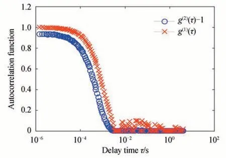
Fig.1 Normalized intensity and electric field ACF for sample 3
2.2 Root-mean-square error of fitted ACF with different data points
By inverting Eq.(4),the fitted ACF can be obtained.The deviation between the fitted ACF and the measured ACF is related to the accuracy of the recovered PSD,and it is usually measured by the fitting error of the ACF.The Root-Mean-Square Error(RMSE)is used to describe the fitting error of the ACF,as shown in Eq.(5)

wheremis the total number of ACF data points involved in the inversion,andg^(1)(τ)=Axis the fitted ACF.
Fig.2 shows theERMSof the ACF shown in Fig.1 as a function of the number of ACF data points used for analysis.Fig.3 shows the fitting residual using 73 and 105 ACF data points in the analysis.It can be seen from Fig.2 that when the number of ACF data points involved in the inversion is smaller than 73,theERMSis relatively small(≤0.003 5)and constant.When the number of points is more than 73,theERMSincreases significantly.This is related to the noise distribution in the ACF data.The measured ACF data has low noise level up to ~73 points and so the value ofERMSis relatively small.There is much more noise in the data after~73 points,and the fitting error increases due to this.As shown in Fig.3,the residual values using 105 ACF data points are greater than that using 73 points.Note that the residual values at longer delay times are obviously greater than those at short delay times when 105 ACF points are used in the inversion,and this contributes to the large increase inERMS.
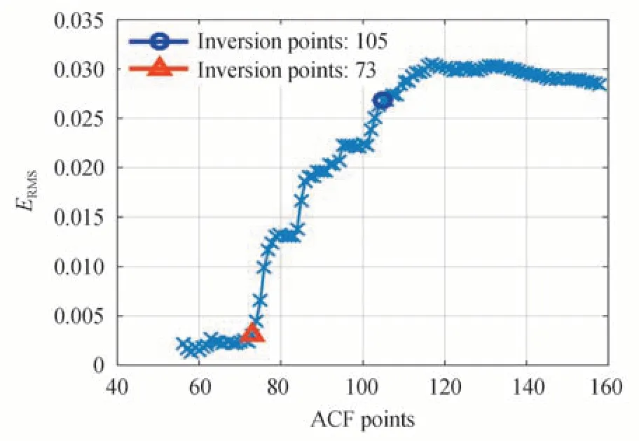
Fig.2 ERMS as a function of the number of ACF data points fitted for sample 3
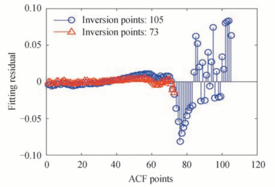
Fig.3 Fitting residuals of the ACF using 105 and 73 data points
The distribution of noise in the ACF shown above suggests that theERMScurve as a function of number of fitted ACF points can be divided into two stages.In the first stageERMSgrows smoothly and the noise level of the ACF is low;while in the second stageERMSgrows rapidly,and the noise level of the ACF is high.Measurement results from samples 1,3 and 4 at different ACF points given in Figs.4(a),4(b)and 4(c)show the same behaviour inERMS.
2.3 The influence of the number of ACF data points on the recovered PSD
The smaller the value ofRN,the more stable the PSD,the smaller the value ofVRSD,the smaller the fluctuation of particle size,and the better the repeatability of the inversion results[15].
The long delay part of the ACF(close to the baseline)has more noise.Fig.5 and 6 respectively show the fitted ACFs and the recovered PSDs for the ACF in Fig.1 for different numbers of fitted ACF data points.Fig.7 and 8 show the stability and repeatability of 60 data sets of this sample for different numbers of ACF points being fitted,and Table 1 shows more inversion results of this sample for different numbers of ACF data points.If too many ACF points are used in the inversion,more noise is introduced,resulting in significant changes in the curvature of the fitted ACF.As shown in Fig.5,taking the fitted ACF within value between 0.96 and 0.92 as an example,there is an obvious difference among the fitted ACF for 105 points,73 points and 59 points.It can also be seen in Fig.6 that the PSD recovered from 105 points deviates significantly from the true PSD,and false peaks are apparent.So when there are too many data points involved,the recovered peak will be inaccurate or false peaks will appear,which will cause the recovered PSD to deviate from the true PSD.It can be seen from Figs.7 and 8 that fitting different numbers of ACF points will affect the stability and repeatability of the results.
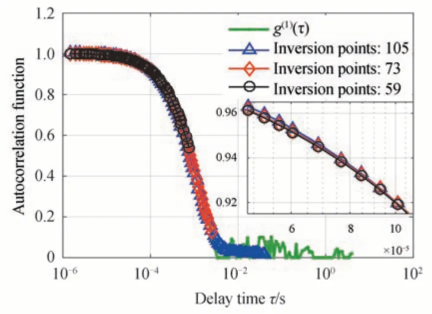
Fig.5 Fitted ACFs for sample 3 with different numbers of ACF data points being fitted
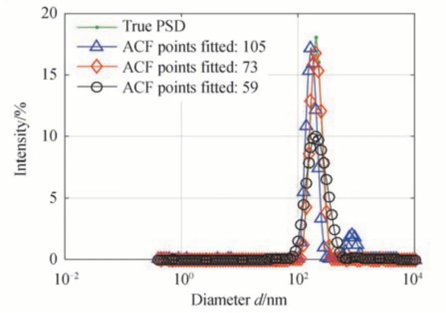
Fig.6 The PSDs of sample 3 recovered with different numbers of ACF data points being fitted
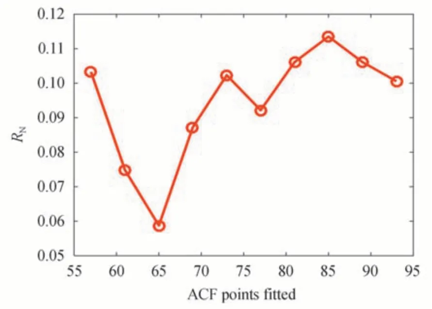
Fig.7 The RN of sample 3 as a function of the number of ACF data points being fitted
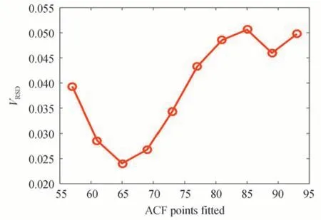
Fig.8 The VRSD of sample 3 as a function of the number of ACF data points being fitted

Table 1 Inversion results of 60 data sets of Sample 3 at different numbers of ACF data points
In summary,if there are too many ACF points in the inversion,the introduced noise will reduce the accuracy of the recovered PSD and false peaks may appear.On the contrary,if too few ACF points are used,sample information may be lost and the results will be inaccurate.Therefore,the key to ensuring the accuracy and stability of the results is how to choose the position to truncate the ACF,in other words,how to determine the optimal number of ACF data points to be fitted.
3 RMSE threshold method
There are two commonly used methods to select the number of ACF points to be fitted.These are choosing a fixed number of ACF points or choosing a fixed ACF level threshold(FACFT).
For the method of a fixed number of ACF points,the same number of ACF points are used for inversion,regardless of the sample.As mentioned earlier,in order to avoid introducing noise near the ACF baseline,the number of ACF points involved in the inversion can not be too many.In this case,for small particles with fast decaying ACFs,fewer ACF points are needed for inversion,while for large particles with slow decaying ACFs,more ACF points are needed.This method can not take both large and small particles into account,so it lacks adaptability,and its inversion results are expected not be optimal.
The FACFT method first sets a specific threshold,then truncates the ACF at the position where the ACF value is less than the threshold,and this sets the number of ACF data points to be used in the inversion.It can be seen from the electric field ACF that there is a lot of noise wheng(1)(τ)<0.1(close to the baseline),so the empirical value of 0.1 is used as the threshold in this paper.Fig.9 shows the selection of the ACF data points by the FACFT method under different noise levels for simulated 100 nm particles.The ACF data were simulated for a log normal distribution with a peak at 100 nm and different levels of random noise was added.As shown in Fig.9,the black ○mark is the position selected by the FACFT method.For the three noise levels of 0.01,0.04,and 0.08,the selected ACF points are 89,89,and 88 respectively,which are basically the same.Clearly,this method does not have the ability to respond to noise and cannot automatically adjust the optimal number of ACF points to be fitted depending on the noise level of the measured ACF data.

Fig.9 The truncation position of the ACF for the two truncation methods at 0.01 level noise,0.04 level noise and 0.08 level noise
In the selection of ACF points,since neither the fixed ACF points nor FACFT method can take into account both the measured particle size and ACF noise level,a different approach is required.In Section 3.2,it was observed that the variation ofERMSwith the number of ACF points fitted can be divided into two stages:in the first stageERMSgrows smoothly;while in the second stageERMSgrows rapidly.The rapid growth ofERMSindicates that the noise contained in the ACF data increases and the reliability of the ACF data decreases with increasing number of data points.The point of inflection of theERMScurve marks where the noise contribution from subsequent data points significantly increases the fitting error and produces poorer inversion results.This is an obvious truncation position,which should effectively select the optimal number of ACF points and avoid the influence of noise in the baseline on the inversion results.Fig.4 shows theERMSvariation with the number of ACF data points being fitted for the various samples.It can be seen from Figs.4(a),(b)and(c)that the position of the rapid growth of eachERMScurve is below 0.003 5.With this in mind,we propose a Root-Mean-Square Error Threshold(RMSET)method as the criterion for selecting the optimal number of ACF data points to be fitted.Furthermore,we set 0.003 5 as theERMSthreshold.

Fig.4 ERMS as a function of the number of ACF data points fitted for Sample 1,Sample 3 and Sample 4
It can also be seen from Fig.4 that the number of ACF points corresponding toERMS=0.003 5 increases as the particle size increases.The red ◇mark in Fig.9 is the selected position using the RMSET method,and the channel number corresponding to this varies with the ACF noise level.The data number of points selected at noise levels of 0.01,0.04,and 0.08 are 101,90,and 83 respectively.It is obvious that more ACF points are selected for an ACF with a lower noise level,while fewer ACF points are selected for one with a higher noise level.This shows that RMSET method is adaptable to noise.The RMSET method has obvious advantages than other methods.It can select the truncation position according to the particle size of the sample and the noise level of the ACF,that is,the larger the particle size to be measured,the more ACF points are used,the smaller the particle size to be measured,the fewer the ACF points,the high-precision ACF takes more ACF points,and the low-precision ACF takes fewer ACF points.
4 Experimental data and analysis
To verify the proposed method,the ACFs for unimodal samples 1 to 5 and bimodal sample 6 were analyzed using the RMSET and FACFT methods and the Tikhonov regularization algorithm for inversion.
Fig.10 shows the truncation positions of the 10 ACFs of sample 3 for the two truncation methods,and Fig.11 shows the corresponding inversion results.Figs.12 and 13 respectively show the fluctuation of the PSD norms and the peak sizes from 60 data sets obtained by the two different truncation methods.The red △and black ☆in the figure mark the truncation positions and inversion results of the RMSET and FACFT methods respectively.It can be observed from Fig.10 that the truncation positions of the RMSET method change due to the fluctuation of noise in the ACFs,while the truncation positions of the FACFT method change little.The fluctuations of the norms and peak sizes of the PSDs obtained by the RMSET method are 7.2%,2.4%,and are smaller than 9.2%,4.6% obtained by FACFT method,as shown in Fig.12 and Fig.13.
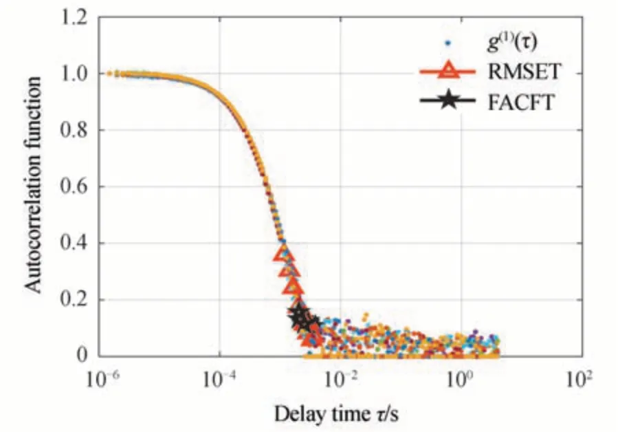
Fig.10 The truncated positions of the electric field ACFs for sample 3 by the two truncation methods
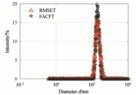
Fig.11 The recovered PSDs of sample 3 by the two truncation methods
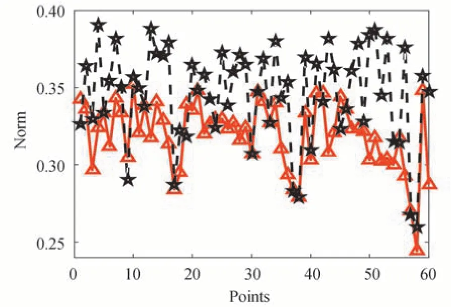
Fig.12 The norms of PSDs of sample 3 from 60 data sets obtained by the two truncation methods
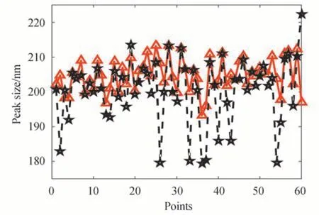
Fig.13 The peak sizes of sample 3 from 60 data sets obtained by the two truncation methods
Table 2 shows the inversion results of 60 data sets of the unimodal samples 1 to 5 obtained by the two truncation methods.It can be seen from Table 2 that for sample 1 and sample 2,theEPKvalues of the two truncation methods are similar and relatively small,and the stability and repeatability of the results of the RMSET method are slightly higher than that of the FACFT method.For samples 3 to 5,theEPK,VRSDandRNof the RMSET method are 2.1%,2.4% and 7.2%,while the FACFT method results are 3.4%,4.6% and 9.2% repectively.It can be seen from the results that for unimodal samples,the RMSET method has higher accuracy,better stability and repeatability than the FACFT method,and the advantages of the RMSET method is more obvious with increasing particle size.

Table 2 Inversion results for different samples under two truncation methods
For bimodal sample 6,theERMSof the 6 data sets for different numbers of ACF data points fitted is shown in Fig.14,and the PSDs recovered by the two truncation methods are shown in Fig.15.It can be seen from Fig.14 that the variation ofERMSwith the number of ACF data points fitted is consistent with the unimodal samples,and the point of inflection ofERMSis below 0.003 5.Therefore,0.003 5 is also set as the threshold,which is same as unimodal samples.The inversion results of RMSET and FACFT methods are shown in Table 3.
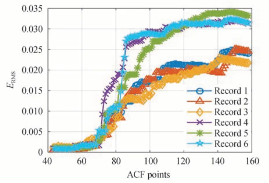
Fig.14 The ERMS of the ACFs at different data points for sample 6
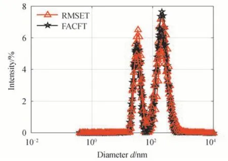
Fig.15 The recovered PSDs of sample 6 by the two truncation methods
In Table 3,Dpeak1andDpeak2are the two peaks of the inversion,EPK1andEPK2are the relative error of the corresponding peak size,VRSD1andVRSD2are the repeatability of the inversion results.According to the experimental data,theEPK1andEPK2values retrieved by the RMSET method are smaller than those of the FACFT method.Also,the values ofVRSD1andVRSD2obtained by the RMSET method are smaller than those of the FACFT method.It is notable that the RMSET method also outperforms the FACFT method in terms of inversion results.

Table 3 Inversion results for sample 6 obtained by the two truncation methods
To summarize,the RMSET method used to select the best truncation position for fitting of the ACF can adapt to different samples and has a certain adaptability to different ACF noise levels.Its flexibility is better than the FACFT method.Moreover,this method is not only suitable for unimodal samples but also for multimodal samples.
5 Conclusion
To improve the accuracy and repeatability of the inverted PSDs,we propose a method to obtain the optimal ACF truncation point by using RMSET,that is,truncate the ACF data fitting at the highest correlation channel which has an RMS error smaller than 0.003 5.The advantage of the RMSET method is that it can automatically obtain the best ACF points according to the measured particle size and ACF accuracy,and it is suitable for both unimodal and bimodal samples.For the measured particles of 203 nm,the relative error of the peak sizeEPK(ie accuracy)obtained by the RMSET method is 2.1%,and the relative standard deviation of particle sizeVRSD(ie repeatability)is 2.4%,which are both smaller than theEPKvalue 3.4% andVRSDvalue 4.6% of the fixed ACF threshold method.The results show that the RMSET method proposed in this paper can effectively improve the accuracy and repeatability of the inversion results,and has an important application value in the field of nanoparticle measurement.

