Forest height mapping using inventory and multi-source satellite data over Hunan Province in southern China

Wenli Huang ,Wankun Min ,Jiaqi Ding ,Yingchun Liu ,Yang Hu ,Wenjian Ni ,Huanfeng Shen

a School of Resource and Environmental Sciences,Wuhan University,Hubei,430079,China

b State Key Laboratory of Remote Sensing Science,Institute of Remote Sensing and Digital Earth,Chinese Academy of Sciences,Beijing,100101,China

c College of Urban and Environmental Sciences,Peking University,Beijing,100871,China

d Academy of Inventory and Planning,National Forestry and Grassland Administration,Beijing,100714,China

e School of Ecology and Environment,Ningxia University,Yinchuan,750021,China

fBreeding Base for State Key Laboratory of Land Degradation and Ecological Restoration in Northwest China,Ningxia University,Yinchuan,750021,China

g Key Laboratory for Restoration and Reconstruction of Degraded Ecosystem in Northwest China of Ministry of Education,Ningxia University,Yinchuan,750021,China

Keywords:Forest canopy height Hunan province Landsat ARD PALSAR-2 Sentinel-1

ABSTRACT Background:Accurate mapping of forest canopy heights at a fine spatial resolution over large geographical areas is challenging.It is essential for the estimation of forest aboveground biomass and the evaluation of forest ecosystems.Yet current regional to national scale forest height maps were mainly produced at coarse-scale.Such maps lack spatial details for decision-making at local scales.Recent advances in remote sensing provide great opportunities to fill this gap.Method:In this study,we evaluated the utility of multi-source satellite data for mapping forest heights over Hunan Province in China.A total of 523 plot data collected from 2017 to 2018 were utilized for calibration and validation of forest height models.Specifically,the relationships between three types of in-situ measured tree heights(maximum-,averaged-,and basal area-weighted-tree heights) and plot-level remote sensing metrics (multispectral,radar,and topo variables from Landsat,Sentinel-1/PALSAR-2,and SRTM)were analyzed.Three types of models (multilinear regression,random forest,and support vector regression) were evaluated.Feature variables were selected by two types of variable selection approaches (stepwise regression and random forest).Model parameters and model performances for different models were tuned and evaluated via a 10-fold cross-validation approach.Then,tuned models were applied to generate wall-to-wall forest height maps for Hunan Province.Results:The best estimation of plot-level tree heights (R2 ranged from 0.47 to 0.52,RMSE ranged from 3.8 to 5.3 m,and rRMSE ranged from 28%to 31%)was achieved using the random forest model.A comparison with existing forest height maps showed similar estimates of mean height,however,the ranges varied under different definitions of forest and types of tree height.Conclusions: Primary results indicate that there are small biases in estimated heights at the province scale.This study provides a framework toward establishing regional to national scale maps of vertical forest structure.

1.Background

Vegetation height is among the top ten variables for tracking biodiversity (Skidmore et al.,2015).Forest canopy height is an important measurement of forest vertical structure that can be used to further model forest biomass (Hurtt et al.,2019).These and other horizontal attributes are essential climate variables to evaluate forest resources and initiate earth system models(Herold et al.,2019;Hurtt et al.,2019).Yet current regional to global scales forest height products lack sufficient spatial or temporal resolutions (Healey et al.,2015).Traditional sample-based forest inventory relies on ground measurements.They use systematic or stratified sampling plots to estimate mean canopy heights at regional to national scales.However,with a limited number of ground samples,traditional forest surveys could not meet the need of accurately mapping the spatial and temporal continuous distribution of forest height at fine resolutions (Duncanson et al.,2019).

Recent advances in remote sensing advocate the mapping of forest canopy heights over large geographical regions at fine resolution.Normally,forest inventory was utilized as calibration and validation datasets for establishing the relationship between forest attributes and various metrics.These metrics include but are not limited to multispectral features and vegetation index calculated from passive optical imagery(Pascual et al.,2010;García et al.,2018;Potapov et al.,2019),CHM(Canopy Height Model)metrics derived from lidar(Light Detection and Ranging) (Hyde et al.,2005;Pang et al.,2008;Simard et al.,2011;Ni et al.,2015),or CCD(Charge-Coupled Device)stereo imagery(Ni et al.,2018;Li et al.,2021),backscattering coefficients and index obtained from SAR(Synthetic Aperture Radar)(Zhang et al.,2017),coherence and phase center heights derived from InSAR (Interferometric SAR) (Kellndorfer et al.,2004;Ni et al.,2014;Qi et al.,2019).Among them,multispectral features from Landsat TM (thematic mapper),ETM+(Enhanced Thematic Mapper plus),and OLI (Operational Land Imager)were often applied for annually long-term analysis(Potapov et al.,2019).Radar features,including ALOS (Advanced Land Observing Satellite-1),PALSAR (Phased Array type L-band SAR),newer generation ALOS-2 PALSAR-2,or Sentinel-1 C-band SAR,were investigated for extracting forest extent stock volume (Hu et al.,2020).In addition,auxiliary data such as topographic and climate variables have been used for continental to the global scale of forest canopy height mapping(Simard et al.,2011;Potapov et al.,2021).The publicly available elevation dataset derived from SRTM (Shuttle Radar Topography Mission),the first spaceborne InSAR mission,has been widely used to generate forest height and biomass maps globally(Simard et al.,2011).

An increasing number of studies explored the estimation of forest structures from field plot-to regional-scales.Previous studies have investigated different parameter or non-parameter approaches,such as simple linear regression (SLR) or multi-linear regression (MLR) (Huang et al.,2013;Sun et al.,2011),regression trees (Potapov et al.,2019),support vector regression (SVR),and random forest (RF) (Kellndorfer et al.,2004;Kellndorfer et al.,2010;Simard et al.,2011).Using multiple independent variables,regression models were found efficient in explaining simple relationships such as maximum tree height between field measurements and lidar-derived CHM (Zhao et al.,2018).For instance,multi-spectral metrics from Landsat Analysis-Ready-Data(ARD)were utilized to build regression models for mapping a 30-m global forest height map (circa 2019) using GEDI (Global Ecosystem Dynamics Investigation) relative height metrics as samples (Potapov et al.,2021).RF or SVR was found to perform better in explaining the non-linear relationship between forest structures such as mean canopy height(Simard et al.,2011) or stock volume (Hu et al.,2020) and remotely sensed multispectral reflectance.For example,multi-spectral features derived from MODIS (Moderate-resolution Imaging Spectroradiometer)and climate variables were used to map forest canopy height globally(Simard et al.,2011).Multispectral features and texture index calculated from Sentinel-2 and PALSAR-2 were used to build RF models for mapping forest stock volume at regional scales(Hu et al.,2020).

Despite many successful explorations in estimating forest structures via remotely sensed data,several critical challenges remain in mapping forest heights over large geographical areas.These include but are not limited to inconsistent spatial and temporal data availability (Potapov et al.,2021),and inaccurate calibration and validation datasets(Simard et al.,2011;García et al.,2018).To this end,we reported here a framework on a subtropical mixed conifer and deciduous forest in China.The main objective of this study was to evaluate the ability of spaceborne remotely sensed data in mapping forest heights seamlessly at fine resolution(30 m)over a large geographic domain.The study site was Hunan Province,the 10th largest province in central China.With variable terrain and mixed forested types,this province was selected as representing southern forest and woodland biomes in the six forest regions over mainland China.Field surveys were conducted as part of the pre-launch calibration/validation campaign for China's Terrestrial Ecosystem Carbon Monitoring(TECM)satellite mission(Hu et al.,2019).The measured plot samples were used to select feature variables from multispectral features,vegetation indices,radar backscattering coefficients,and topographic indices.Then,forest height models were calibrated and validated using field measured samples.Last,the forest height maps generated from this study were validated against existing forest canopy height products.The development of a wall-to-wall province scale map of forest height will be of great significance for future studies over broader geographical domains.

2.Methods

Our methodology consists of four major components (shown in Fig.1):1) field data preparation;2) remote sensing and ancillary data processing;3)model development and evaluation;and 4)province scale mapping and evaluation.

2.1.Study area and field data

2.1.1.Study area

The domain of study was the Hunan Province,China,located at latitude 24.64°-30.13°N,longitude 108.78°-114.25°E,covering a land area of approximately 211,855 km2.The domain represents Chinese southern subtropical forest that exhibits diverse canopy structures,various vegetation phonologies,and abundant biodiversity.Located in a transition zone between the middle and lower reaches of two river basins(the Yangtze River and the Xiangjiang River) and a plateau platform(Yungui Plateau),the region has a unique geographical landscape.It has a clear seasonality and a warm and humid climate.The annual average temperature ranges from 16°C to 18°C,total precipitation varies between 1200 and 1700 mm,and the frost-free period ranges from 216 to 269 days.

The forested area covers 59.82%of the land area in Hunan(Statistics,2019).According to the statistics from the 8th National Forest Inventory,Hunan Province is the region with the largest proportion of forest resources in the southern forest region.These cover 131 forest units recorded by the State Forestry Administration.Ten dominant tree species and forest types include cypress (Cupressus funebrisendl.),oak (Quercusspp.),Masson's pine(Pinus massonianaLamb.),Chinese fir(Cunninghamia lanceolata),slash pine (Pinus elliottii),poplar group (PopulusL.),camphorwood and Chinese timber nanmu,coniferous mixed,and broad-leaved mixed.The region features mountainous and rolling topography.Elevations range from 30 to 1150 m.Together the region thus presents all challenges and opportunities encountered in mapping forest vertical structures.

2.1.2.Field data collection

The Hunan forest field survey was prepared as one of the core prelaunch field campaigns for the TECM satellite mission.A total of 523 circled plots(in a 15-m radius)were surveyed from October 2017 to April 2018 (purple circled dots shown in Fig.2).These plots were collected under a sampling design to represent major forest types and across different classes of canopy cover and tree height in Hunan Province.These plots cover the ten major forest types in the province,where each forest type is divided into 15 type units (5 tree height classes and 3 canopy classes).Four sample plots with a projection radius of 15 m were investigated for each type of unit.Within each type unit,sample plots were selected at least 200 m apart on the same slope,slope direction,or distance.Within each sampled plot,a set of measurements were taken,including the location of the plot center,individual tree locations,height,density,crown size,and diameter at breast height(dbh).The locations of the plot center and individual tree were taken through the combined use of the Differential Global Positioning System (DGPS) and Global Navigation Satellite System (GNNS).This new technology provided a geolocation accuracy ranging from 0.1 to 0.25 m(Hu et al.,2019).

2.1.3.Plot height calculation

The height of a tree is a quantitative indicator reflecting the growth status of a tree,and it is also an important basis for reflecting the stand quality of forests.Within our sampled plot,all individual trees were measured.Therefore,various types of tree height were prepared,including maximum height and average height.First,maximum tree height(Hmax)within a plot was calculated by getting the maximum tree height within the plot:

whereHiis the height of the individual tree,the unit is meter.

Then,average heights were prepared.In forestry,it is usually divided into the average height of stand (AHS) and average top height (HT) for various purposes.Commonly used AHS in forestry,calculated based on field measurements are conditional average height,weighted average height,and dominant average height(Thomas and Harold,2001).Using our measured tree data,two types of AHS were calculated,averaged-and basal-area-weighted tree height,respectively.

The average tree height(Havg)was calculated by averaging individual tree heights:

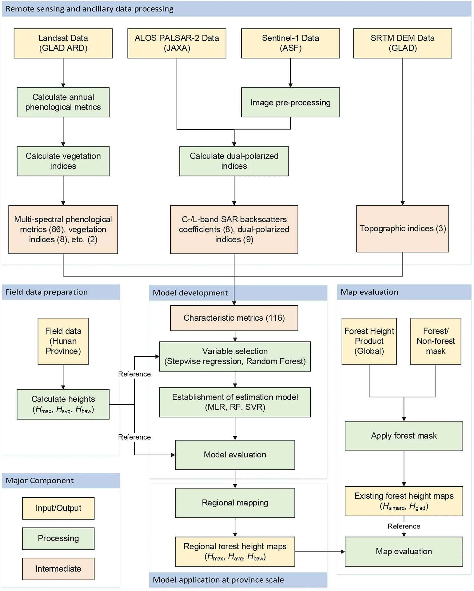
Fig.1.The diagram of data preparation,modeling,validation,mapping,and evaluation framework.

Fig.2.Study area showing general land cover classes (forest,non-forest,and water),and locations of sampled field plots in Hunan Province,China.General land cover classes are taken from the Finer Resolution Observation and Monitoring of Global Land Cover (FROM-GLC,2017) dataset.

wherenis the number of trees within the plot.

Then,basial-area-weighted height (Hbaw) was calculated by weighting the tree heights by basal area(BA)as follows:

whereBAiandDBHiare the basal area (BA) and diameter at the breast(DBH) for tree numberi.

Summary statistics of the field plots are given in Table 1.The plot number of different forest types ranged from 33 to 61.The maximum tree heights have a mean of 19.1 m,ranging from 3.8 to 43.1 m.The average tree heights have a mean of 12.4 m,ranging from 3.0 to 38.4 m.The basal-area-weighted tree heights have a mean of 14.5 m,ranging from 3.0 to 39.1 m.

2.2.Remote sensing data

2.2.1.Multispectral metrics from landsat

Annual normalized multispectral metrics were prepared from Landsat Analysis Ready Data(ARD).First,the ARD product was acquired from the website supported by Global Land Analysis and Discovery team(GLAD),where 16-day Landsat surface reflectance (SR) were composited from Landsat TM,ETM+,and OLI data downloaded from USGS.The preprocessing step contains radiometric calibration,atmospheric correction,geometric refinement,and filling of data gap (cloud and shadows) with the values from previous observation within 4 years (Potapov et al.,2020).Then,ARD annual phenological metrics (i.e.,type B used in this study) were prepared through the GLAD Landsat ARD Tools V1.1(https://glad.umd.edu/ard/glad-landsat-ard-tools),containing a set of normalized spectral reflectance,vegetation indices,and statistical measurements of the abovementioned values.These include spectral reflectance from blue (B),green (G),red (R),near-infrared (NIR),shortwave infrared (SWIR1) and mid-wave infrared (SWIR2),land surface brightness temperature(LST),and vegetation index such as normalized ratio of NIR and red(RN),NIR and SWIR1(NS1),NIR and SWIR2(NS2),spectral variability vegetation index(SVVI)(Table S1).

Besides,statistical measurements of the abovementioned indices were computed,such as minimum (min.),maximum (max.),quantiles(Q1 to Q4),averaged values between min and Q1 (avmin25),averaged values between Q3 and max(av75max),averaged values between Q1 and Q3 (av2575).Then,additional statistical measurements of the abovementioned original reflectance sorted by reference values (NDVI,NS2,and LST)were computed.A set of 36 metrics were calculated,including minimum(min),maximum(max)of original reflectance sorted by NDVI,NS2,and LST(Table S2).

Moreover,additional vegetation indices (VI),Tasseled Cap (TC)indices,and topographical indices were prepared (Table 2).Enhanced VIs(i.e.,EVI and EVI2),ratio VI(RVI),and TC indices(TCB,TCG,TCW,and TCWGD) (Crist,1985) were calculated from normalized Landsat ARD metrics.Topographical indices such as elevation,slope,and aspect of the corresponding pixel were calculated from STRM data.Details about Landsat ARD normalized reflectance and phenological metrics could be referred to Hansen et al.(2008)and Potapov et al.(2020).

To cover the Hunan Province,1610 Landsat ARD tiles from the year 2015-2017 were first downloaded,processed to 35 1°×1°degree tiles,then mosaiced and clipped to the province boundary.A false-color composite (red for SWIR1,green for RED,and blue for NIR) mosaic of Landsat data was given in Fig.3a.

2.2.2.L-band SAR metrics from PALSAR-2

Annual L-band radar metrics were prepared from ALOS-2/PALSAR-2 L-band SAR imagery.PALSAR-2 annual mosaic in the year 2017 was processed by Japan Aerospace Research and Development Agency(JAXA).This dual-polarized(HH and HV)SAR backscattering coefficient(ortho and slope corrected) was organized as 1°× 1°tiles in approximately 25 m(0.00022°)spatial resolution(JAXA,2018).Data stored in digital number (DN) were converted to gamma naught (γ°) values in decibel unit(dB)using the following equation:

where,CFis a calibration factor (-83.0 dB for PALSAR-2 mosaic data),and 〈〉 represents the ensemble averaging.A multi-look was applied to reduce speckle noise.Then,the image was rectified and terrain-corrected using 90 m SRTM dem(Shimada et al.,2014).Details could be referred to the dataset description document Ver.H (JAXA,2018).For this study,a total of 35 1°×1°scenes in the year 2017 were downloaded,mosaiced,and clipped to the province boundary(Fig.3b).The definition of metrics and tile name convention could be referred to in Table 3 and Table S3.

2.2.3.C-band SAR metrics from Sentinel-1

Annual C-band radar metrics were prepared from Sentinel-1 SAR imagery.Sentinel-1 data from the year 2017 was accessed from Alaska Satellite Facility(ASF)via python API.The dual-polarized (VV and VH)Interferometric Wide swath(IW)Ground Range Detected(GRD)products were chosen,where each scene has a swath of 180 km and a spatial resolution of 5 m × 20 m.For efficiency in data processing and index computation,a 1°× 1°tiling system was designed following the ARD gridding system.Within each tile,the same orbit data products were first calibrated and assembled using modules provided by the Sentinel Application Platform(SNAP).Then,the data were multi-looked to 20 m using a 2×2 window to reduce the speckle noise.A“Refined Lee Sigma”speckle filter was applied during the pre-processing.Finally,terrain correction was conducted using local incidence angles and processed to gamma naught(γ°).Lastly,statistical indices such as mean,median,and standard deviation of a pixel over the field time domain(i.e.,Oct 2017 to Apr,2018) were calculated (Table 2).To cover the province,a total of 250 Sentinel-1 GRD products were downloaded and processed to 35 1°×1°tiles,and mosaiced(Fig.3c).The definition of metrics and a list of tiles were summarized in Table 3 and Table S3.

Table 1 Summary statistics of field plots.Plot distributed by ten major forest species,the corresponding number of field plots,numbers of trees,maximum tree height(Hmax),averaged tree height (Havg),and basal-area-weighted height (Hbaw).

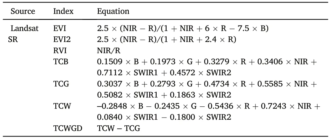
Table 2 Summary of additional vegetation indices derived from Landsat multispectral surface reflectance sorted by reflectance values.

2.2.4.Characteristic metrics from the multi-source dataset

A total of 116 characteristic metrics was prepared from the abovementioned multi-source spaceborne satellite data,including 96 multispectral and vegetation metrics (Table 2,Tables S1 and S2),17 SAR backscatter coefficients,and indices (Table 3),and 3 topographical metrics.Specifically,the averaged values of each metric were extracted from the metric raster over sampled field plots using the precise circled boundary.To reduce the error caused by the plot geolocation and resampling process,a 1-m raster analysis size was set in the“Zonal Statistics”function provided by ArcGIS®.

Table 3 Summarized definitions of PALSAR-2 and Sentinel-1 SAR metrics.

2.2.5.Forest/non-forest masks

Existing land cover maps were utilized to differentiate between forested and non-forested areas for forest height estimations at the province scale.Three global landcover maps,including FROM-GLC 2017(Finer Resolution Observation and Monitoring of Global Land Cover at 30-m resolution,2017v1)(Gong et al.,2013),GlobeLand30 2020(30-m resolution Global Land Cover,2020 version) (Chen et al.,2021) and GLC-FCS30 2020 (Global Land Cover with Fine Classification System at 30 m in 2020)(Liu et al.,2020),were used to generate three sets of forest masks.These maps classified 10 Level-1 land cover types and their definitions of forest varied.FROM-GLC defined“forest”as areas dominated by trees greater than 3 m in height and with greater than 15% total vegetation cover.The GlobeLand30 is a 30-m resolution global land cover data product.GlobeLand30 defined“forest”as land covered with trees where top density is over 30%,and deciduous broadleaf forest,evergreen broadleaf forest,mixed forest,and open woodland with a tree cover 10%-30%(Chen et al.,2015).GLC-FCS30 defined“forest”as land with trees greater than 3 m and with tree cover greater than 15%(Zhang et al.,2021).Original landcover data were downloaded from the Earth Science System (ESS) data center at Tsinghua University (http://data.ess.tsinghua.edu.cn/fromglc2017v1.html),National Geomatics Centerof China (http://globallandcover.com/),and Zendo(10.5281/zenodo.4278952).

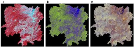
Fig.3.Statewide false-color composite mosaic of(a)Landsat(R:SWIR1,G:Red,B:NIR;averaged values between minimal and maximum quantiles),(b)PALSAR-2(R:HH,G:HV,B:HH/HV;averaged values),and(c)Sentinel-1(R:VV,G:VH,B:VH/VV;averaged values)over the Hunan Province.(For interpretation of the references to color in this figure legend,the reader is referred to the Web version of this article.)

2.2.6.Existing maps of forest canopy height

Two global scale forest canopy height maps,Simard et al.(2011)and Potapov et al.(2021)were prepared for map evaluations(Table 4).The Simard et al.(2011)was a spaceborne lidar derived global canopy height map (hereafterHsimard) at 1-km spatial resolution (～0.0083°).It was developed using GLAS measured maximum canopy height (RH100)collected from the year 2003-2009 as a reference,and 7 spatial predictor variables,including elevation(SRTM+GTOPO),tree cover(MOD44B),and climate variables (precipitation and temperature fromWorldclim).The Potapov et al.(2021)was a prototype global canopy height dataset in approximately 30-m spatial resolution (0.00025°) developed by the GLAD team(hereafterHglad).It was generated by combining information from space-borne lidar measured height and Landsat data.Specifically,the GEDI height metric(relative height at 95%,RH95)was first validated airborne LiDAR data and then were integrated with Landsat ARD phenological metrics in 2019 to build forest height models.Eventually,multi-year forest canopy heights were inversed using time-series ARD metrics,allowing the detection of forest height changes.

2.3.Model development and evaluation

2.3.1.Feature variable selection

Characteristic variables were selected and analyzed from the multisource remote sensing dataset using all field measurements as a reference.Two sets of experiments were conducted to select feature variables for modeling three types of forest height (i.e.,Hmax,HbawandHavg).Altogether,a total of 12 variable combination scenarios were designed to cover the case of using a single sensor,multi-sensor,vegetation index,and topographical index (Table 5).First,initial variables were selected via a both-direction stepwise regression.Using AIC(Akaike information criterion) as criteria,the stepwise regression picked the best subset of variables by iteratively evaluating the performance of the model,while adding or removing variables in the prediction model at the same time.Second,feature variables were chosen using a packaged method (i.e.,Variable Selection Using Random Forests,VSURF).Briefly,the random forest used two-third of bootstrap samples for constructing trees and nodes,and the remaining samples for calibration of“out-of-bag”estimates(Breiman,2001).Using out-of-bag(OOB)error as the criteria,the VSURF selected a suitable subset of variables that have a close relationship with forest heights and low internal redundancy.In addition,multiple linear regression (MLR) models were applied to describe the relationship between tree heights and the independent variables.Variable selection and regression model analysis used the R package‘MASS’and‘VSURF’(Genuer et al.,2015;R Development Core Team,2016).

Table 4 Summary of two global forest canopy height products.

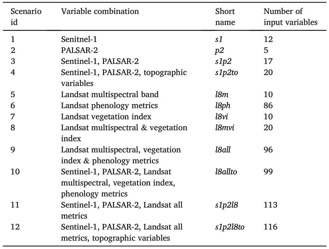
Table 5 Different scenarios of input variable combinations for forest height modeling.

2.3.2.Height model calibration

We developed models to predict three types of forest heights (i.e.,Hmax,HbawandHavg) as a function of selected characteristic variables.Explicitly,we tested three types of model,including multiple linear regression (MLR),support vector regression (SVR),and random forest(RF).Critical parameters within these models were tuned through running multiple times.For SVR,model parameters such as the epsilon(ε)and the cost value(c)were optimized,by a grid screening ofcranges from 22to 29and ε ranges from 0 to 1.The radial basis function (RBF)was set as the kernel function.For the RF model,the important model parameters include the number of trees to grow(ntree)and the number of variables randomly sampled as candidates at each split(mtry).A similar screening,ntreeranges from 500 to 2000 andmtryvalues range from 1 to 12,was set up to select the best parameters.The modeling and analysis process used the R package‘MASS’,‘randomForest’,‘e1071’,respectively(R Development Core Team,2016).

2.3.3.Height model validation

After getting tuned model parameters,a 10-fold cross-validation approach was adopted for model validation and evaluation.The 10-fold cross-validation approach split the plots into 10 sets.Each time,9 sets were used as the calibration dataset and the rest was left as the validation dataset.The process was repeated 10 times,and the average performance was calculated.The model performances were evaluated and the best model was determined.Specifically,statistical indicators,including coefficient of determination (R2),root mean squared error(RMSE),and relative error (rRMSE),were employed to validate results using the plot data as the reference.wherexiis theith value from field measurements,yiis the predicted value from the statistical model;iis the sample index;andis the mean value of field measurements;andnis the sample size.

2.4.Province scale mapping and product evaluation

2.4.1.Province scale mapping of forest height

The tuned models were then used for wall-to-wall mapping of forest heights(i.e.,Hmax,Hbaw,andHavg)in Hunan Province for the year 2017.Each height model using different independent variables was applied to all 35 tiles over the domain.Particularly,the model of maximum tree height (Hmax) was applied to metrics in the year 2019 to match the timeframe ofHglad.All forest height maps and forest/non-forest masks were mosaiced,and re-projected to a common frame of reference to minimize the distortion in the area.

2.4.2.Map product comparison

Map estimates of forest heights from this study were compared to available map products at the province scales.Maximum,mean,and standard derivation of forest heights were compared between measurements from in-situ plots and estimates from map-based results.These include averaged values over the forested area from maps generated in this study(Havg,Hbaw,andHmax)and two global maps(HsimardandHglad).Additionally,forest/non-forested masks generated from three global land cover data products (GLC_FCS30,2020,FROM-GLC,2017;and Globe-Land30,2020)were used to assist the evaluation of map-based results.

3.Results

3.1.Characteristic of multi-source satellite metrics

The characteristic of metrics was analyzed through linear correlation analysis.Results show that the correlations between in-situ measured tree heights and multi-source metrics were moderately weak (rranged from 0.10 to 0.45)(Table S4).The low to moderate correlations between multi-source metrics and forest heights reflected the fact that multispectral reflectance,C-band or L-band SAR backscattering coefficients have a different level of saturation to canopy height due to limited penetration.Top multispectral metrics from Landsat that have a high negative correlation with tree heights are the minimum value of red and green band (l8rmin,l8gmin),the average value between the minimum and first quantile of the green and red band (l8g25min andl8r25min),and the average annual value of green band(l8g).

The top vegetation indices from Landsat that have a positive correlation with tree heights are the tassel cap indices (l8tcwgd,l8tcw,andl8tcb),the average annual value of ratio vegetation index (l8rvi),enhanced vegetation index (l8evi2),and normalized differential vegetation index (l8ndvi).The correlation between variables from Sentinel-1(s1vhsd,s1vh,s1vhmd,s1vvsd),PALSAR-2 (p2hv,p2hh),and SRTM DEM(elevation,slope)and in-situ tree heights are comparably lower than those values from Landsat multispectral bands(Table S4).

3.2.Variable selected for forest height modeling

Two variable selection approaches,stepwise regression and VSURF package,were compared in feature variables selection for modeling forest heights.Among hundreds (116) of independent variables,approximately 40 were selected by stepwise regression (Table S8) and around 10 were chosen by the VSURF(Table S9).

The best variable combinations selected by the stepwise regression method(Table S10;Table S8)were“l8allto”forHmax,“s1p2l8to”forHbaw,and“s1p2l8”forHavg,respectively.Among three types of forest height,RF model selected variables were mainly from Landsat multispectral reflectance and phenology metrics,topographic variables,and radar metrics.These variables include SRTM DEM(elevation,slope),minimum quantile of Landsat spectral bands (green,red,blue,shortwave nearinfrared),and PALSAR-2 L-HV polarization (p2hv).Then,the selected variables were used in SVR models.The optimal parameters ofcand ε for SVR models were 4 and 0.18 forHmax,8 and 0.14 forHbaw,and 8 and 0.49 forHavg,respectively.Although the rank of variables from Sentinel-1 (s1vv,s1vhmd,s1vvsd,s1npdimd),PALSAR-2 (p2hv),and SRTM (elevation,slope) are relatively low,these vaeviriables were selected by stepwise regression in all three cases.

The best variable combinations selected by the VSURF method(Table S10;Table S9) were“l8allto”forHmax,“s1p2l8to”forHbaw,and“s1p2l8to”forHavg,respectively.Among three types of forest height,RF model selected variables were mainly from Landsat multispectral reflectance and phenology metrics,topographic variables,and radar metrics.These variables include SRTM DEM(elevation,slope),minimum quantile of Landsat spectral bands (green,red,blue,shortwave nearinfrared),and PALSAR-2 L-HV polarization(p2hv).The optimal parameters ofntreeandmtryfor RF models were 1000 and 6 forHmax,500 and 3 forHavg,500 and 4 forHbaw,respectively.

After data standardization,the absolute value of the coefficient of the independent variable can reflect its influence on the height prediction model (Table S5-S7).The top three variables that had the greatest influence are the enhanced vegetation index (l8evi2orl8evi),the average annual value of blue band(l8b)and shortwave 2 bands(l8sw2),and the average value between third quantile and maximum of the shortwave red band(l8sw175smax).

3.3.Forest height model evaluation using plot data

Height models built by different variable scenarios were evaluated using the 10-fold cross-validation approach through two statistical indicators (rRMSEandR2).The model performances in the calibration stage (Fig.4) and validation stage (Fig.5),were grouped by three modeling approaches (upper,middle,and bottom row),and the twovariable screening methods (stepwise regression in left,and VSURF package in right).Within each subfigure,therRMSE(filled bars)andR2(dotted lines) were plotted for three types of forest height in different colors,and sorted by 12 variable scenarios from left to right.Among different variable combinations,the coefficient of the determinant (R2)increased,while the relative error(rRMSE)decreased with the increasing number of the sensor and metrics.

Then,the best models selected from different variable combinations were summarized in Table 6.Evaluation using plot data showed that RF models performed the best among all three types of height models(Table 6).In the calibration stage,three models (MLR,RF,and SVR)explained moderated to high variability (0.47-0.93) in tree heights.RF models had the best performance compared to the two other models(MLR and SVR).Among three different height models,theRMSEof the best RF models is 2.3,1.8,and 1.7 m for three types of heights (Hmax,Hbaw,Havg).The second was the SVR model,and the MLR model was the worst.

In the validation stage,RF models also showed the best generalization ability.Results indicated that all three models (MLR,RF,and SVR)explain low to moderated variability(0.33-0.52)in tree heights.The RF model explained the highest variability inHavg(R2=0.52,RMSE=4.2 m,rRMSE=29%).Then followed byHmax(R2=0.50,RMSE=5.3 m,rRMSE=28%),andHbaw(R2=0.47,RMSE=3.8 m,rRMSE=31%).In both cases,results indicated that RF models have the best performance compared with the other two models (MLR and SVR).Therefore,RF models were selected to conduct the regional mapping of forest canopy heights over the Hunan Province.

3.4.Height maps comparison to existing products

The RF-derived map of forest height maps(Havg,Hbaw,andHmax)from this study were compared to two existing height products over the Hunan province.In general,all heights map products followed similar patterns in topography (Fig.6a SRTMelevation) and landscape (Fig.6b FROMGLC,2017).While the fine-scale comparison in a mountainous area showed larger disagreements among different forest canopy height maps(Fig.7).

At the province scale,the estimated forest heights showed a large difference among different maps (Table 7).The mean estimates fromHsimardhad a slightly higher value (13.2 ± 13.7 m) compared toHglad(12.5±4.6 m),andHavg(12.6±2.7 m),but lower thanHmax(19.0±3.8 m in 2017,and 19.0±3.0 m in 2019)andHbaw(14.2±2.8 m),and the maximum heights from in-situ plot data(19.1± 7.7 m).

4.Discussions

Our study systematically explored mapping forest heights by fusion of in-situ measured tree heights and multi-source satellite data.Various combinations of characteristic variables for forest height models were tested through stepwise regression and VSURF approaches.Three types of tuned regression models were calibrated,validated,and applied for mapping of maximum-(Hmax),averaged-(Havg)and basal-area-weighted tree height (Hbaw) over the study site.The analysis highlighted several important aspects,concerning the quality of reference samples,selection of feature variables and models,the sensitivity of multi-source metrics on forest heights,the strategy of model evaluation,other factors on highresolution forest height mapping,and directions of future research.

4.1.High-quality plot data

Accurate plot geolocation and precise tree height measurements guaranteed a solid reference dataset.On one hand,this study collected precise plot center locations using DGPS and GNSS with a measurement error of less than 0.5 m (estimated 0.1-0.25 m in the best case).Thus,small geolocation errors within in-situ plots avoided mismatch between the field plot and corresponding remote sensing metrics (Huang et al.,2013;Hu et al.,2020).On the other hand,the plot-level forest heights were aggregated from individual tree heights.These accurate height measurements thus formed a solid calibration and validation dataset for forest height model development.

Although this study was carried out by combining in-situ measurements and passive optical and radar metrics,the findings may also be useful for forest height inversion using lidar data as samples.Recent studies indicated that the position accuracy error of GEDI footprints leads to the deviation of height products,and its correlation between plot-level aboveground biomass was improved after position correction (Wang et al.,2019).

4.2.Exploration for feature variable selections

This study used two variable selection approaches,stepwise regression,and VSURF,to screen variables for different forest height models.Results showed that stepwise regression (Table S8) always selects more variables than VSURF (Table S9).The subsequent model evaluations indicated VSURF has advantages in selecting more concise feature variables.However,in terms of method efficiency,our experiments confirmed that stepwise regression is faster than VSURF.This is reasonable as the RF model has higher complexity than the multivariable linear model,leading to a lower efficiency especially under a large number of variables.

Table 6 Model evaluation using the 10-fold cross-validation approach.

Fig.4.Sensitivity of rRMSE (%) and R2 of three models (RF in the top row;SVR in the middle row;and MLR in bottom row) to variable scenarios during the calibration stage using two variable selection methods (VSURF in left column,and stepwise regression in right column).Maximum tree height (Hmax in green color),basial-area-weighted height (Hbaw in blue color),and average height (Havg in orange color).(For interpretation of the references to color in this figure legend,the reader is referred to the Web version of this article.)

Evaluation results grouped by sensors also showed a limited improvement in model accuracy.No matter what type of learning model is used,only Landsat metrics or all-radar metrics could be trained with high accuracy in the calibration and validation stages (Figs.4 and 5).Landsat metrics alone achieved model accuracy close to that of all categories(optical,radar,and topo),indicating the capacity of using Landsat data for mapping forest heights large scales(Potapov et al.,2021).

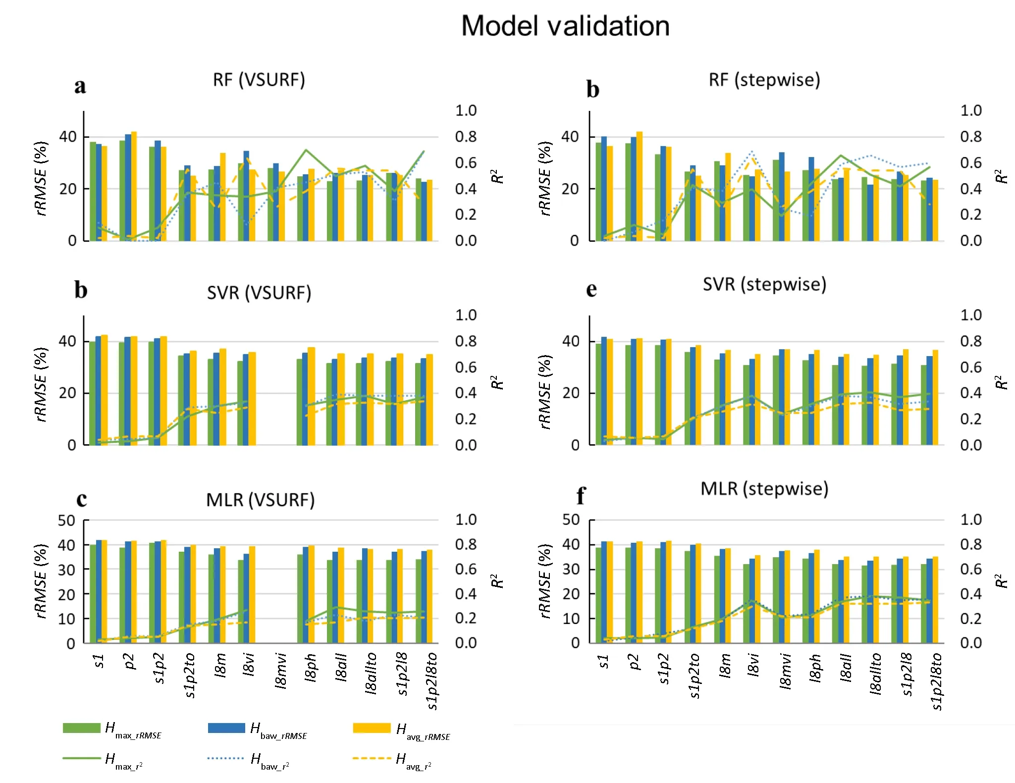
Fig.5.Sensitivity of rRMSE(%)and R2 of three models(RF in the top row;SVR in the middle row;and MLR in bottom row)to variable scenarios during the validation stage using two variable selection methods(VSURF in left column,and stepwise regression in right column).Maximum tree height(Hmax in green color),basial-areaweighted height(Hbaw in blue color),and average height(Havg in orange color).(For interpretation of the references to color in this figure legend,the reader is referred to the Web version of this article.)

In addition,the comparison between different Landsat metrics found some unexpected results.Using annual spectral metrics,the model accuracy is better than the ones that use vegetation index.This is explainable as the spectral metrics were related to vegetation growth and environment conditions that are widely used in the large-scale mapping of forest canopy height(Simard et al.,2011;Mahoney et al.,2016).

4.3.Sensitivity of multi-source satellite metrics to forest heights

The first highlight of our objective is to utilize multi-source satellite data for the estimation of forest heights.Model evaluation results indicated the sensitivities of passive optical and radar data to forest height varied,confirming that their different sensitivities to forest structural parameters (Kellndorfer et al.,2004).While multi-temporal metrics made up for this disadvantage to a certain extent(Potapov et al.,2019).Thus,multispectral variables were selected many times in all cases that involve Landsat metrics.Similarly,the C-band and L-band radar backscatter have different penetration degrees.Thus,L-band SAR metrics from PALSAR-2 always showed a higher correlation coefficient and significance than of C-band metrics from Sentinel-1(Tables S5-S7).

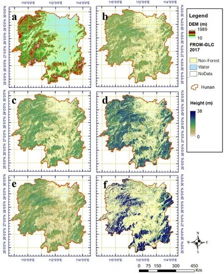
Fig.6.Province scale maps of Elevation (a), Havg (b), Hbaw (c), Hmax (d), Hpotapov (e),and Hsimard (f) at 30-m spatial resolution.

Grouping variables by a sensor,there are similar findings and interesting phenomenon.Firstly,variable combinations from multi-source sensors are better than indicators from a single sensor.Previous studies also found that fusion of passive optics and radar is better than single category(Sun et al.,2011).Secondly,our experiments indicated that the optical indicator is better than the radar or terrain indicator.The Landsat-derived combinations,including reflectance,vegetation indices,and phenological indicators,are better than radar metrics.In addition,elevation has a good correlation with forest height.This phenomenon has been reported in previous studies,especially over the mountainous area(Simard et al.,2011).As SRTM utilized a C-band InSAR instrument,and the contribution from vegetation is not completely separated from ground elevation,thus the elevation may contain partial vegetation height.

4.4.Model evaluation approach

This study adopted a 10-fold cross-validation method to evaluate three sets of height models (MLR,SVR,RF).This choice is made after a comparison to 70%-30% data with-holding approach (hereafter 70-30 approach),in which model performance (Table S10).Evaluation result from the 70-30 approach showed similar however lower accuracy than the 10-fold approach,especially for the RF model ofHbaw(rRMSEis～4.0%higher).A one-time split of reference samples is less stable due to sampling bias under a small sample situation.Suggestion from this study is that the 10-fold cross-validation method should be adopted for the RF model when the sample size is relatively small to feature characteristic variables.

Table 7 Comparison of estimated forest heights over Hunan Province.

In either evaluation case,the comparison between different models showed that the RF model could explain a moderately higher variability in tree heights,compared with the other two models (MLR and SVR).Model evaluations also indicated that in either approach,the RF models have the best performance in calibration-and validation stages.Therefore,the RF model is recommended for height modeling using multisource metrics,consistent with previous studies (Simard et al.,2011;Mahoney et al.,2016).

4.5.Framework of high-resolution forest height mapping

The second highlight of our objective is to set up a framework for mapping forest heights seamlessly at 30-m spatial resolution.To complete this goal,we adopted a 1°×1°map framing system following the Landsat ARD(Potapov et al.,2019).PALSAR-2 and Sentinel-1 data were re-organized into 1°× 1°tiles with a spatial resolution of 0.00025°per pixel in the WGS84 geographical system (Table S3).For the PALSAR-2 annual mosaic,the original resolution is 0.00022°(～25 m).For Sentinel-1 IW data,the original resolution is 5 m × 20 m.Thus,the resampling into 0.00025°slightly multi-looked the radar backscatter coefficients.Overall,this map framing system greatly facilitates batch processing and large-scale data handling.

Previous studies indicated that the choice of forest/non-forest masks may have influences on the mean estimates in the map-based product(Huang et al.,2017).Our investigation also found large variances in the estimates of forest coverage in Hunan province(ranged from 49.69%to 62.02%).These estimates were from China Statistic Report (49.69%)(2018),Hunan Statistic Report (59.69%) (2019),GLC_FCS30 2020(53.49%),GlobeLand30 2020(55.99%),and FROM-GLC 2017(62.02%).However,the variances in estimates of forest heights were relatively small and within the standard deviations (Table S11).Thus,we finally chose FROM-GLC 2017 that had a close date to our product,an overall accuracy of 72.43%,and consistent classification schemes cross-walked to existing land-cover systems (Gong et al.,2013,2019),to generate the reference forest/non-forest masks for the province scale forest height estimation.

4.6.Limitations and potential improvements

Future work will focus on improving the quality of metrics,incorporating lidar samples,and exploring a deep learning approach.Firstly,this study used Landsat annual composites from multiple years of observation,thus some areas were affected by Landsat ETM+strips issues and terrain effects.Similar data issues were found in PALSAR-2 and Sentinel-1 SAR annual mosaics.Higher quality of multi-source metrics could further improve the accuracy of the height model.Second,a relatively limited number of in-situ plot samples(523)were used.Within this in-situ dataset,few low or high height values were sampled,leading to overestimations in low-height areas and underestimations in higherheight areas.Similar issues were reported in the mapping of forest aboveground biomass (Huang et al.,2017).Incorporating national inventory plots as well as space-borne lidar acquisitions (GEDI,ICESat2,and TECM)could leverage these issues(Dubayah et al.,2020;Duncanson et al.,2019).Lastly,model performance may be further improved through the fusion of deep learning and machine learning algorithms that take advantage of information mining and the ability of regression modeling.

5.Conclusions

This study explored the high-resolution (30 m) mapping of forest heights at a regional scale combining inventory data and multi-source satellite remote sensing data.Three types of statistical learning models were evaluated,including multiple linear regression (MLR),support vector regression (SVR),and random forest (RF).Height models were calibrated and validated using field plots to predict forest height as a function of characteristic variables.Maximum,basal-area-weighted,and averaged tree heights (i.e.,Hmax,HbawandHavg) were mapped over the Hunan Province (211,855 km2).

Plot-level analysis revealed low to moderate correlations between insitu measured tree heights and characteristic metrics from multispectral and radar data.However,through a combination of multiple characteristic metrics,the machine learning models performed better in predicting plot-level forest heights.Overall,the characteristic variables that have a relatively stronger correlation with forest heights include topographic variables (elevationandslope),Landsat multispectral reflectance (green,red,blue,shortwave near-infrared),and PALSAR-2 cross-polarization backscatters (p2hv).The accuracy evaluations using 10-fold crossvalidation showed that the RF models achieved moderately good estimation accuracy(R2ranged from 0.47 to 0.52,RMSEranged from 3.8 m to 5.3 m,rRMSEranged from 28% to 31%) when the correlations between feature variable and height are not strong (rranged from 0.1 to 0.45).All three forest height maps have general consistency with existing map products over the study domain.The forest height mapping framework proposed in this study could support further national scale mapping of forest structures such as height and biomass.

Authors’contributions

WH and WM contributed equally to this work.WH,YL,and HS designed experiments.WM,JD,and YH processed and analyzed datasets.WH wrote the initial manuscript with contributions from all co-authors.All co-authors participated in discussing and interpreting the results of the research.

Funding

This work was funded by the Open Fund of State Key Laboratory of Remote Sensing Science (OFSLRSS201904),National Natural Science Foundation of China(41901351),Start-up Program of Wuhan University(2019-2021),and Natural Science Foundation of Ningxia Province(2021AAC03017).

Ethics approval and consent to participate

Not applicable.

Consent for publication

Not applicable.

Availability of data and material

The datasets used and generated from this study are available from the corresponding author on reasonable request.

Competing interests

The authors declare that they have no competing interests.

Acknowledgments

We greatly acknowledge the support from the Academy of Inventory and Planning under collaboration for China's Terrestrial Ecosystem Carbon Monitoring(TECM)satellite mission.We also appreciate the Global Land Analysis and Discovery (GLAD) team,Alaska Satellite Facility(ASF),Japan Aerospace Research and Development Agency(JAXA),and Tsinghua University,for providing Landsat ARD,PALSAR-2 mosaic data,Sentinel-1 SAR data,and FROM-GLC landcover dataset free of charge.

Appendix A.Supplementary data

Supplementary data to this article can be found online at https://do i.org/10.1016/j.fecs.2022.100006.