A graphics processing unit-based robust numerical model for solute transport driven by torrential flow condition*

Jing-ming HOU, Bao-shan SHI†‡, Qiu-hua LIANG, Yu TONG, Yong-de KANG,Zhao-an ZHANG, Gang-gang BAI, Xu-jun GAO, Xiao YANG

1State Key Laboratory of Eco-hydraulics in Northwest Arid Region of China, Xi’an University of Technology, Xi’an 710048, China

2School of Architecture, Building and Civil Engineering, Loughborough University, Loughborough LE11 3TU, UK

3Northwest Engineering Corporation Limited, Xi’an 710065, China

Abstract: Solute transport simulations are important in water pollution events. This paper introduces a finite volume Godunovtype model for solving a 4×4 matrix form of the hyperbolic conservation laws consisting of 2D shallow water equations and transport equations. The model adopts the Harten-Lax-van Leer-contact (HLLC)-approximate Riemann solution to calculate the cell interface fluxes. It can deal well with the changes in the dry and wet interfaces in an actual complex terrain, and it has a strong shock-wave capturing ability. Using monotonic upstream-centred scheme for conservation laws (MUSCL) linear reconstruction with finite slope and the Runge-Kutta time integration method can achieve second-order accuracy. At the same time, the introduction of graphics processing unit (GPU)-accelerated computing technology greatly increases the computing speed. The model is validated against multiple benchmarks, and the results are in good agreement with analytical solutions and other published numerical predictions. The third test case uses the GPU and central processing unit (CPU) calculation models which take 3.865 s and 13.865 s, respectively, indicating that the GPU calculation model can increase the calculation speed by 3.6 times. In the fourth test case, comparing the numerical model calculated by GPU with the traditional numerical model calculated by CPU, the calculation efficiencies of the numerical model calculated by GPU under different resolution grids are 9.8–44.6 times higher than those by CPU. Therefore, it has better potential than previous models for large-scale simulation of solute transport in water pollution incidents. It can provide a reliable theoretical basis and strong data support in the rapid assessment and early warning of water pollution accidents.

Key words: Solute transport; Shallow water equations; Godunov-type scheme; Harten-Lax-van Leer-contact (HLLC) Riemann solver; Graphics processing unit (GPU) acceleration technology; Torrential flow https://doi.org/10.1631/jzus.A2000585 CLC number: TV131.2

1 Introduction

In recent years, many flash floods caused by severe rainstorms have occurred. For instance, in March 2019, during a period of heavy rain, a severe storm occurred in Papua Province in Indonesia, and the massive flood claimed 63 lives. In July 2012, an unpredictable rainstorm killed 79 people in Beijing,China. Flash floods caused by such heavy rains occur frequently around the world. Because of the acuteness and unpredictability of heavy rains, they bring tremendous damage to human life and economy. The impact of flash floods on cities is extremely important (Barredo, 2007; Roccati et al., 2019; Bayazıt et al., 2021). In cities, such flood events can destroy chemical plants and wastewater treatment plants.Such an event may threaten the water safety of urban and rural residents and affect the water quality of downstream rivers and lakes. Understanding the contaminant transport process is thus of fundamental and practical importance in hydraulic and environmental engineering (Wang and Cheng, 2002; Zhao et al., 2007; Zhang et al., 2010; Duarte et al., 2013).Under these circumstances, a strong and efficient model is needed to predict the track of point-source pollutants transported by flood-driven water.

Water pollution incidents have occurred frequently, causing the deterioration of water quality in rivers and lakes, leading to serious eutrophication,and threatening the survival of fish (Tao et al., 2012;Li et al., 2018; Chen et al., 2021). Because of frequent pollution incidents, mastering the process of pollutant transport in water bodies plays an important role in water conservancy projects and environmental and ecological engineering (Kachiashvili et al., 2007; Liu,2011; Zhang, 2011; Bi et al., 2013; Tang et al., 2015).Through the establishment of high-efficiency and high-precision numerical models, the hazard range and duration of water pollution accidents can be quickly determined, and then effective measures can be taken to reduce the harm caused by the accident.The surface hydrodynamic process is mathematically described by a 2D shallow water equation, and a shallow water solver is used to establish an efficient and high-precision numerical model to study its motion (Audusse and Bristeau, 2003; Murillo et al., 2009;Hou et al., 2018a; Dong, 2020). However, the Boltzmann equation can also be used to establish numerical models for many fluid mechanics problems(Aidun and Clausen, 2010; La Rocca et al., 2015; Liu et al., 2020; Venturi et al., 2021). The advantage of this method is that it does not require the solution of large-scale nonlinear partial differential equations,which considerably simplifies the calculations. La Rocca et al. (2020), using discrete Boltzmann equations, developed a method for simulating transcritical shallow water flow, and verified the validity of the model through numerical and experimental results.Many shallow-water solute transport models have been reported in recent years and most of these adopt the Goundnov-type scheme to establish a robust numerical model. For example, Begnudelli and Sanders(2006) proposed a high-resolution unstructured grid finite volume algorithm for simulating 2D unsteady water flow and material transport, and analyzed the effects of different slope limiters on its calculation accuracy and efficiency. Benkhaldoun et al. (2007)established a self-adaptive mesh-based pollutant transport model with high computational accuracy,but the scheme did not fully satisfy total variation diminishing (TVD) characteristics. Kong et al. (2013),based on a high-precision finite volume model that solves the transport motion equation on an unstructured grid, used the operator-splitting method to calculate the material convection flux and introduced a gradient limiting factor to ensure the TVD characteristics of the calculation format and to reduce the numerical oscillation caused by the large concentration gradient of the material. Petti and Bosa (2007) developed an accurate 2D Eulerian numerical method for the prediction of pollutant transportation in a natural water body. Their model uses a non-uniform grid to discretize the computational domain, which may pose challenges to large-scale calculations. Thus, it is not easy to design an accurate and efficient numerical model for solving shallow water and solute transport equations. At the same time, the problems of a large amount of calculations and a low calculation efficiency must be faced (Song et al., 2014). Efficient and accurate numerical modelling thus provides a significant tool for environmental impact management and water project design for water pollution incidents.

In this study, the authors aim to resolve the shallow flow-driven solute transport problem by considering all the above challenging issues and presenting a graphics processing unit (GPU)-accelerated model for dry-bed simulations over a complex domain. The model solves a 4×4 matrix form of the hyperbolic conservation laws consisting of 2D shallow water and solute transport equations. The monotonic upstream-centred scheme for conservation laws (MUSCL) format, with second-order spatiotemporal precision, was used to ensure calculation accuracy and avoid numerical oscillation (Hou et al.,2014). Second-order spatial reconstruction and nonnegative depth reconstruction methods improve the accuracy of the model and meet the TVD characteristics (Hou et al., 2013a). The accuracy and efficiency of the model are tested by several cases. The numerical format provides a well-balanced solution and maintains non-negative water depth and solute concentration in applications involving wet and dry complex areas. The model ensures computational accuracy while increasing computational efficiency.Therefore, it has better potential than previous models for large-scale simulation of problems in the real world.

2 Governing equations and numerical methods

2.1 Shallow water equation and transport equation

Shallow flow hydrodynamics and passive solute concentration transport are described by the shallow water equation and the depth-averaged advectiondiffusion equation, respectively. In vector form, the shallow water and advection-diffusion equations may be written as a 4×4 matrix:

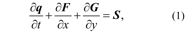
wheretis the time;xandyare the Cartesian coordinates;qis the flow variable vector;FandGare the flux vectors in thexandydirections, respectively;Sdenotes the vector of the source terms. The vectors may be given as follows:

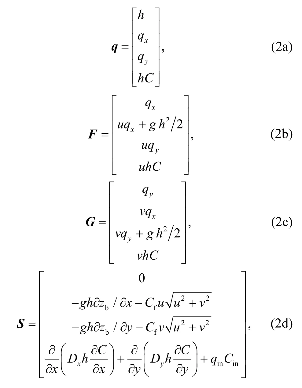
wherehis the water level;uandvare the depthaveraged velocity components in thexandydirections, respectively;Crepresents the solute concentration;qx=uhandqy=vhare the unit-width discharge in the two Cartesian directions;hCis the solute volume per unit area;grepresents the acceleration due to gravity;zbis the bed elevation;Cfis the bed roughness coefficient determined by the Manning coefficientsnandh, which has the formgn2/h1/3;DxandDyare thexandycomponents of the solute diffusion coefficientD, respectively;qinis the flow intensity of the point-source solute;Cinis the average concentration of the solute perpendicular to the point-source. In addition, the water levelη, which equalsh+zb, is also used in this study.

2.2 Numerical method

2.2.1 Finite volume model

Using the cell-centred finite volume method, the integral form of Eq. (1) over a control cell is written as

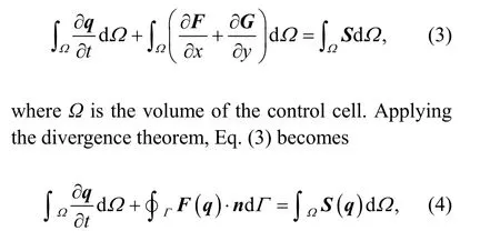
whereΓis the boundary of the grid;nis the normal vector outside the unit perpendicular to the boundary of the grid and is defined by [nx,ny]T;F(q)·nis the flux at the grid boundary and is expressed as

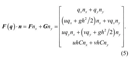
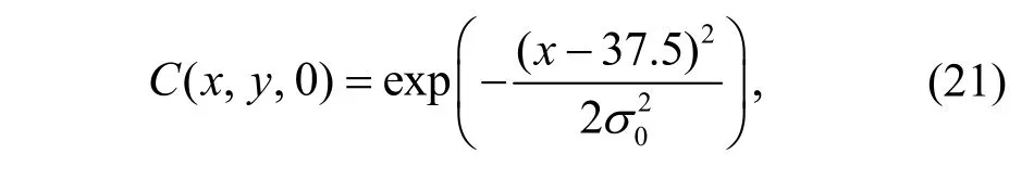
The line integral for theF(q)·ntotal edges of the square grid is expressed by algebraic equation as

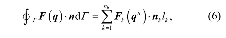
wherekis the index of a side of a cell;lkis the side length of thekth side of the cell;nbis the number of cell boundaries;Fk(qn) is the interface flux of the four interfaces of the unit grid–east, west, south, and north–including the mass flux, momentum flux, and solute flux;nkis the outer normal direction of the four interfaces.

In Eq. (4), the first term on the time derivative uses the difference method. From timento timen+1,theqvalue of the cell is updated to

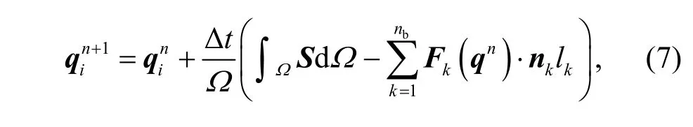
whereq=[h,qx,qy,hC]Tis a conservation variable,which includes water depth variables, flow variables,and solute variables; Δtis the calculation time step,which needs to meet the Courant-Friedrichs-Lewy(CFL) condition limit. The detailed calculation process is described in reference (Hou et al., 2013a);Fis the hydrodynamic transport flux;Sis the source term approximation, which includes the bottom slope source term and friction source term; for the specific processing method, please refer to Hou et al. (2013b).When updating the solute concentration, a minimum water depth should be set (10−6m in this study). When the cell grid water depth is less than the minimum water depth, the solute concentration is 0.

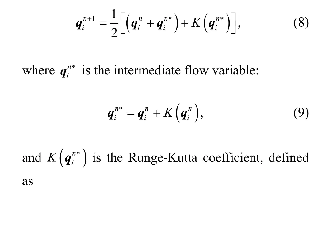
To obtain a second-order numerical scheme with a time factor, the Runge-Kutta time integration method is employed, and the time-matching Eq. (7)may be rewritten as

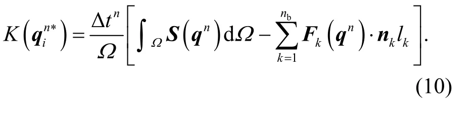
2.2.2 Flux calculation

The model uses the Harten-Lax-van Leer-contact(HLLC)-approximate Riemann solver to calculate the hydrodynamic force and transport flux, which has a strong ability to capture shock waves. It was implemented successfully in (Liang, 2010; Hou et al., 2013a,2014, 2018b). This method can effectively mitigate situations of excessive numerical damping or severe numerical oscillation caused by the transport advection term. It can deal well with the changes in the dry and wet interfaces in an actual complex terrain. In this study, the coupled shallow water and advectiondiffusion equations are considered, and hence, the HLLC solver should be used. Here, to calculate the grid edge fluxes, eastFk(q)·nkcan be obtained with this solver as (Kawahara and Umetsu, 1986)

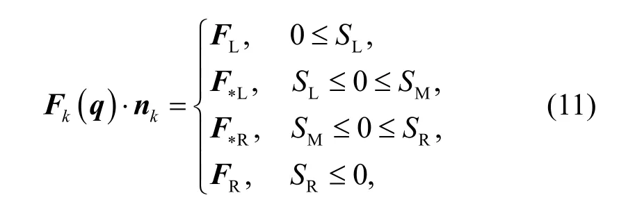
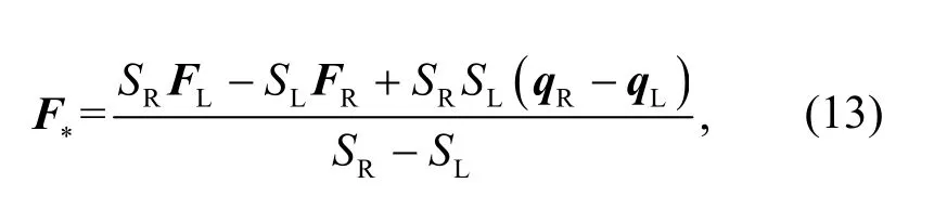
whereFL=F(qL)·nkandFR=F(qR)·nkare calculated from the left and right Riemann states;SL,SM, andSRare the left, middle, and right wave speeds, respectively;F*LandF*Rare the fluxes in the left and right middle regions of the HLLC solution structure and are calculated as

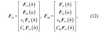
wherevLandvRare the tangential velocities, andCLandCRare the substance concentrations.F*LandF*Rare calculated from the Harten-Lax-van Leer (HLL)formula (Harten et al., 1983):

whereSL,SM, andSRare the left, middle, and right wave speeds in the HLLC Riemann solution structure.Fraccarollo and Toro (1995) recommended the following formulae for estimatingSL,SM, andSRto facilitate applications in wetting and drying:

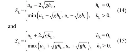
For the middle wave speedSM, Toro (2001) suggested the following choice:

2.2.3 GPU-accelerated computing The dynamic wave methods and Godunov-type schemes have been successfully applied in many studies, but the available computing power limits their application in many areas of high-resolution representation. The GPU parallel computing technique offers a new approach to such simulations. The GPU’s highly parallel structure makes it more efficient than central processing units (CPUs) for algorithms. The compute unified device architecture(CUDA) programming language is used to implement the GPU parallel computing technique. The CUDA programming model uses the CPU as the host and the GPU as the coprocessor or device. The CPU is responsible for processing logical transactions and serial calculations. The GPU is responsible for performing parallel processing tasks. When the model starts to run calculations, data is first read into the host (main memory), and then the data of the grid information, initial boundary conditions, calculation parameters, etc. are initialized in each cell. The corresponding GPU device space is allocated to copy the data to the device (video memory). After the computation is completed, the result is synchronously copied back to the main memory. The implementation is detailed in the authors’ previous studies (Smith and Liang, 2013; Liang et al., 2016;Hou et al., 2020). The successful and efficient implementation of the GPU computing technique is shown in Fig. 1. If the data exchange between CPU memory and GPU memory is too frequent, the data exchange delay will reduce program performance.Therefore, to avoid frequent data exchange in the output process of the results, the calculation time is extended. In the calculation of efficiency comparison in this study, the results will be output only after the simulation ends.

3 Results and discussion

The proposed numerical scheme for shallow flow-driven solute transport is validated against several benchmark tests and results and alternative numerical predictions, using different types of GPU computers for large-scale calculations, and comparing the results with those of CPU calculations. The Courant number for the CFL condition is set to 0.5, andg=9.81 m/s2andρ=1000 kg/m3. The solute is assumed to maintain the same density as water.

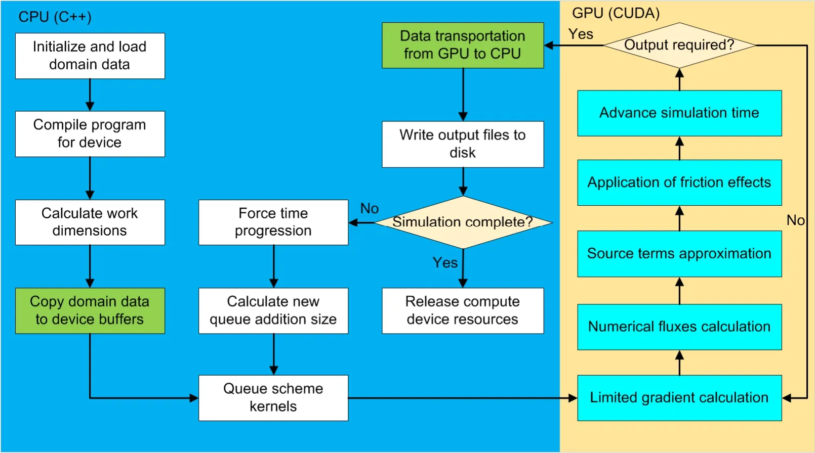
Fig. 1 Flowchart of the computation using GPUs

3.1 Pure solute advection verification

The first test case is characterized by advection of solute clouds in a stable uniform flow. The model is verified by advection in a uniform flow field using a square solute cloud. The assumed computing domain is an open channel with a slope of 10°, a length of 1000 m, and a width of 200 m. The computational domain covering the channel is divided into 1000×200 cells with a size of 1 m×1 m. The left and right boundaries are the inflow and free outflow conditions. The north and south boundaries are set to closed. In the whole domain, a constant flow field is achieved by setting the hydrodynamic parameters.That is, a depth of 0.1 m is imposed in the computational domain. The 40 m×40 m solute cloud is placed in the channel with a central coordinatex=100 m. The value of the concentration for the solute cloud is assumed to be 3 mg/L. If the transport solute performs only advection motion on the water flow, the advection motion control equation is given as

These conditions are also shown in Fig. 2a. A simulation time step of 1 s and a total time of 2000 s are adopted in this case. The contour and position distributions of the simulated solute cloud transport results att=600 s andt=1000 s are shown in Figs. 2b and 2c, respectively. Theoretically, due to the neglect of the diffusion term, the solute cloud maintains its initial profile and concentration at all times in the flow field. However, numerical dissipation is inevitable. Although numerical dissipation still exists,Fig. 2 shows that the dissipation is very small and that the concentration field deformation is relatively small.Therefore, the advection term processing method used in this model has a high accuracy and can achieve a high accuracy in practical applications.

3.2 Simulation of solute diffusion under hydrostatic conditions

3.2.1 Setting the initial conditions of the model

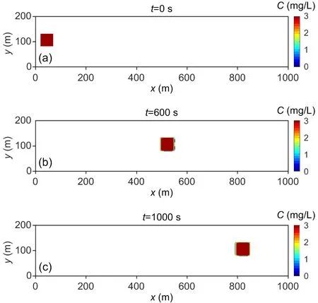
Fig. 2 Initial computational domain (a), and the solute cloud locations with a constant concentration profile at t=600 s (b) and t=1000 s (c)

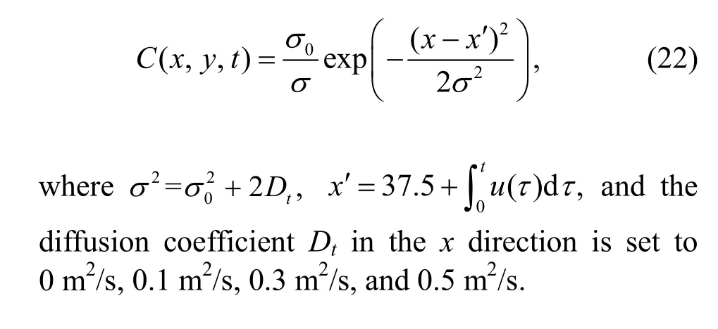
The characteristic of this test case is the diffusion of solute clouds under hydrostatic conditions. The harmony of the model and the appropriateness of the solute diffusion term are verified. Withh=1 m,u=0,andv=0, the 2D diffusion equation for this idealised case is given as This test case is similar to the transport problem with Gaussian distribution of concentration peaks(Shao et al., 2012). The length and width of the calculation domain are 75 m and 30 m, respectively. The computational domain is divided into 150×60 cells with a size of 0.5 m×0.5 m and a frictionless domain with a horizontal bed. The simulation is calculated with the time step Δt=1 s, and the total calculation time is 300 s. In the whole calculation process, the four boundaries are closed boundaries, with the initial condition of concentration given as

whereσ0is the standard deviation of the Gaussian distribution and is set to 1 m.

“Come, little sister,” said the other princesses; then they entwined their arms and rose up in a long row to the surface of the water, close by the spot where they knew the prince’s palace stood

The analytical solution of the solute concentration distribution at any time is

To quantitatively analyze the simulation results,error method diagnostics are employed to measure the accuracy. The lower the ERR is, the closer the result is to the exact solution.CiandCexactare defined as the numerical and exact solutions, respectively, and ERR is defined as

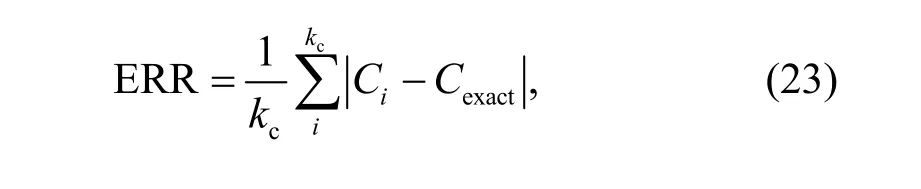
whereiis the cell number, andkcdenotes the total number of cells.

3.2.2 Discussion of the simulation results and accuracy analysis

Fig. 3 shows the results att=300 s. During the long calculation period, the calculated water level of the model does not change and remains at 1 m, which is consistent with the analytical solution; the flow velocity is always maintained at 0. Therefore, the model has good harmony, and no false flow occurs.

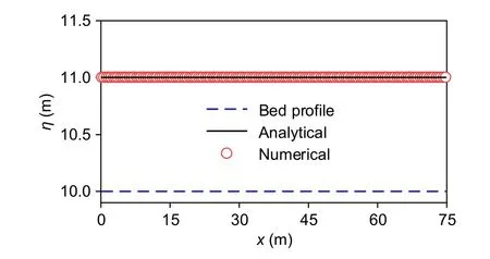
Fig. 3 Solute diffusion under hydrostatic conditions:comparison of the numerical and analytical water surface elevations along the x direction at the centre of the computed domain line at t=300 s

The concentration peak transport process is calculated for diffusion coefficientsDof 0 m2/s,0.1 m2/s, 0.3 m2/s, and 0.5 m2/s. A comparison of the numerical solution and the analytical solution att=10 s is shown in Fig. 4. Fig. 4a shows the results ofD=0 m2/s (the initial concentration distribution). The numerical method in this study can also obtain stable and reasonable results, and the calculated results before and after the solute cloud concentration peak are in good agreement with the analytical solution.Figs. 4b–4d show that as the diffusion coefficient increases, the concentration peak decreases, the distribution width increases, the concentration peak becomes increasingly flat, and the numerical solution and analytical solution are better fitted. Table 1 shows that the error is small at different times under different diffusion conditions. It is clear that the numerical method adopted maintains the highest accuracy by holding the closest shape to the analytical result. This indicates that the model can effectively reduce numerical damping and has high precision and good stability.

3.3 Simulation of dam-break flow and solute transport with uniform concentration

Proposed by Kawahara and Umetsu (1986), this case is often used to check the calculation accuracy of the model and the effectiveness of the dynamic dry and wet boundary treatment. The calculation domain is a rectangular area of 75 m×30 m, and the bottom topography is calculated by

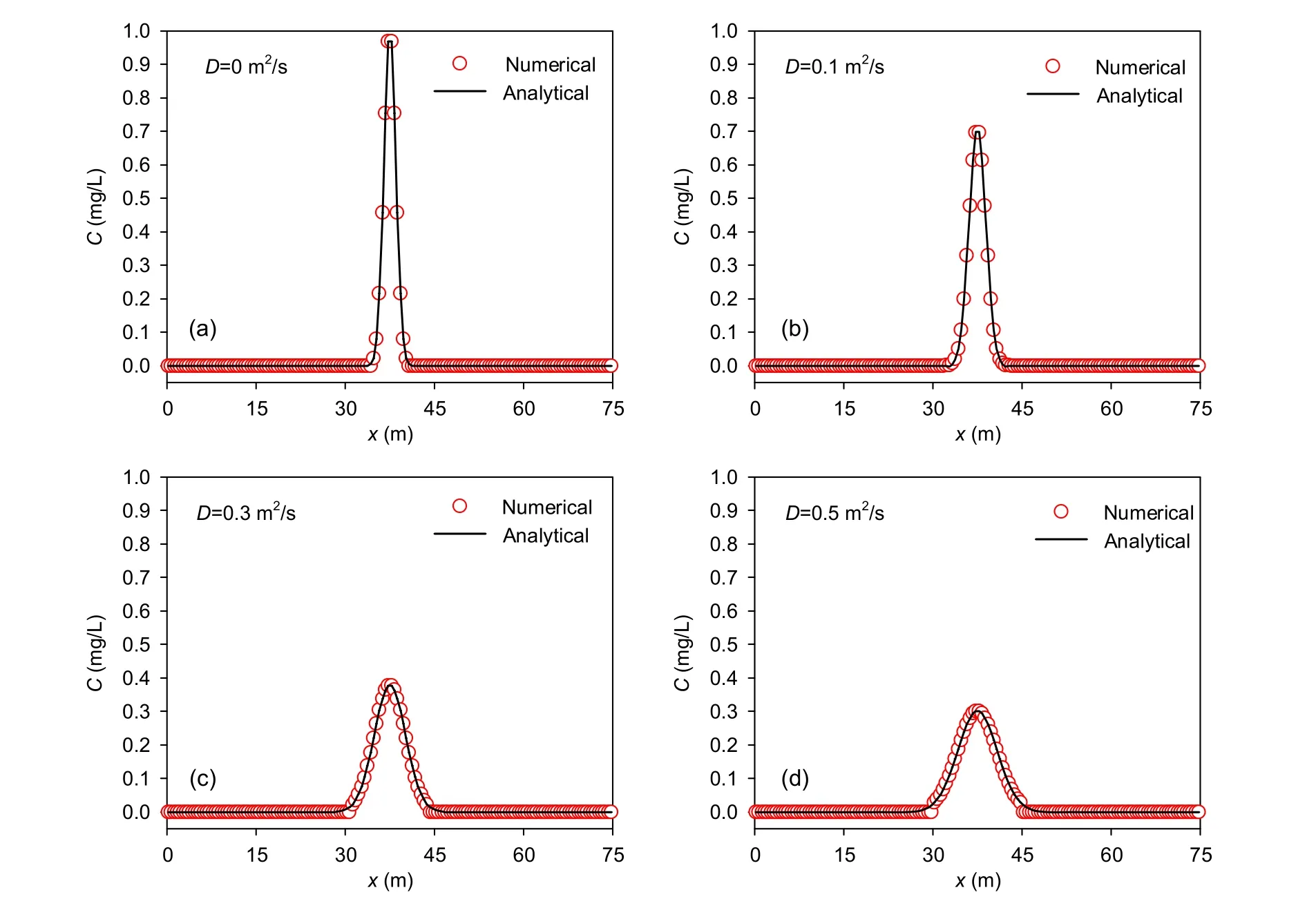
Fig. 4 Solute diffusion under hydrostatic conditions: the concentration curve along the x direction, comparing the numerical and analytical solutions

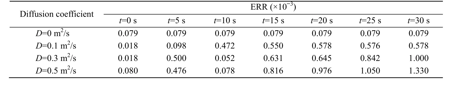
Table 1 ERRs of 2D diffusion equations

An infinitely thin dam is located atx=16 m, and divides the area into an upstream reservoir and a downstream dry flood area. The still water depth upstream of the dam is 1.75 m. It is contaminated by a solute mixture with a concentration of 1 mg/L. The Manning roughness coefficientn=0.018 s/m1/3is assumed throughout the domain. The computational domain is discretized into 150×60 regular square grids. The four side walls are closed boundaries. The movement of the solute does not consider material diffusion or degradation during transport. We assume that the dam is removed immediately att=0, and that the total duration of the entire simulation calculation is 300 s.

Fig. 5 shows the results att=2 s in terms of a 3D surface plot and contours for both water depth and solute distribution. After the dam break, the polluted water rushes into the downstream area, and att=2 s,the flood front reaches two small humps and begins to climb. Theoretically, because diffusion is neglected,the concentration of the solute is always 1 mg/L in the wet region and 0 in the dry region. The simulation results are consistent with the facts, as shown in Figs. 5c and 5d. Therefore, the solute concentrations at the dry and wet edges are correctly simulated, and no obvious numerical diffusion is observed. Due to the large momentum generated by the dam break, the water continues to flow downstream rapidly. The dam-break water infiltrates and passes through the two small humps aftert=6 s, as shown in Fig. 6. After hitting the large hump, the water begins to climb up the large hump. Due to the blocking effect of the large hump, only part of the water can pass through the boundary wall near the southern and northern ends of the large hump and continue to flow downstream; this flow direction is shown in Fig. 6e. The leading edge of the solute concentration coincides with the dry-wet interface. A reliable and effective numerical model is established. As shown in Fig. 7, att=12 s, the dam-break water flows downstream through the front portion of the large hump to reach the downstream end of the calculation area. Due to the interaction between the dam-break water and the hump, a shock wave in the opposite direction is generated, and the water flow propagates both downstream and to the upstream boundary, as shown in Fig. 7e. Fig. 8 (p.845)shows the results att=30 s. It can be seen from the figure that the current reaches the eastern boundary.Since the dam-break wave collides with the east boundary to generate waves in the opposite direction,the water flow moves upstream, as shown in Fig. 8e.This wave-topography-boundary interaction continues until the momentum of the dam break is dissipated by the bed friction. Eventually, the flow becomes static once more, where the tops of the three humps are dry again. The Godunov-type scheme is observed to correctly capture the complex flow patterns induced by the dam-break wave (shock) interacting with the three humps and the domain boundaries. The numerical results are the same as those reported by Liang (2010) on a uniform grid and those reported on the adaptive grid by Zhang et al. (2015).For the GPU and CPU high-resolution numerical models on an NVIDIA Tesla M 1080 GPU computer,it took 3.875 s and 13.875 s, respectively, to complete the 300-s dam water flow evolution process on 9000 computing grids. Liang (2010) and Zhang et al. (2015)reported that the time required to complete the simulation on 16 000 uniform grids or adaptive grids was 277.3 s and 101 s, respectively. Therefore, for this more practical simulation calculation, the GPU’s parallel computing efficiency is more obvious and it maintains a similar accuracy.

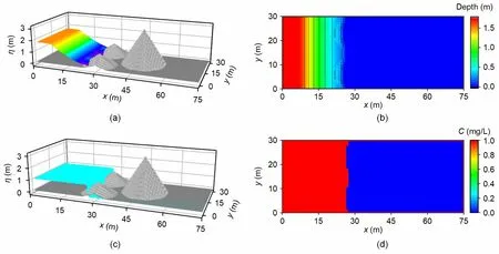
Fig. 5 Dam-break flood evolution: numerical results at t=2 s

Fig. 6 Dam-break flood evolution: numerical results at t=6 s

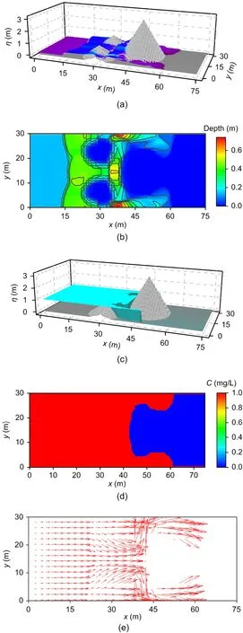
Fig. 7 Dam-break flood evolution: numerical results at t=12 s

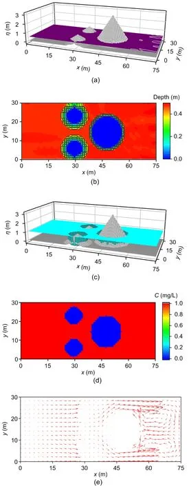
Fig. 8 Dam-break flood evolution: numerical results at t=30 s

3.4 Point-source solute transport driven by the Malpasset dam break

The French Malpasset dam was built in 1956,had a maximum storage capacity of 5.5×107m3, and was mainly used for agricultural irrigation and urban water use. Due to continuous heavy rain at the end of November, 1959, the Malpasset dam water level rose rapidly in a short period of time. The dam finally broke at 21:14 on December 2, and the dam break was rapid. It can be considered a transient dam separating the Malpasset reservoir and the downstream terrain, as shown in Fig. 9. The dam-break water flows rapidly downstream and eventually enters the sea. The sea surface elevation is 0 m, the water level upstream of the dam before the dam break is 100 m,and the downstream water depth is 0 m. Hypotheticalpoint source given byqin=1 m/s andCin=1 mg/L is set at (9281 m, 5244 m). The solute diffusion coefficient is 0.5 m2/s, and the river Manning coefficient is taken as 0.033 s/m1/3. The terrain data use digital elevation model (DEM) data with a resolution of 10 m (1.5 million square grid cells). The GPUaccelerated high-resolution model is used to simulate the dam-break water flow evolution that drives the solute transport process, and the simulation time is 3000 s.

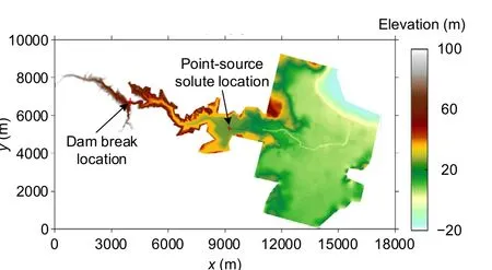
Fig. 9 Malpasset dam break: the topographic numerical elevation, dam break position, and point-source solute position

Fig. 10 shows the results att=1000 s andt=1800 s in terms of water depth. After the dam break,the water flow rapidly evolves downstream and then reaches the downstream plain, as shown in Fig. 10b.The numerical simulation results are the same as those reported by Hou et al. (2013b) for the dam-break water flow evolution on unstructured grids. The Godunov scheme can correctly capture the complex flow caused by the interaction of dam-break waves with the complex terrain. Fig. 11 shows the results of the solute concentration distribution at different times.After the simulation starts, the flood reaches the solute release source att=900 s, as shown in Fig. 11a.Aftert=900 s, the solute is transported to low-lying places with the flood. During the simulation, it was observed that the water depth profile matches the solute distribution profile, which indicates that drastically changing floods can cause large-scale water pollution and rapidly affect downstream water bodies after destroying solute-releasing facilities. At all output times, the solute transport process of the flood-driven point source is very similar to that obtained by Cao et al. (2019).

3.5 Simulations for different grid resolutions and their efficiencies

Different resolutions of the Malpasset terrain were used to simulate the dam-break flood-driven point-source solute transport based on the test case in Section 3.4. The elaborate computational grid leads to an increase in the number of grid squares, which seriously affects the calculation efficiency of the model and may even make it impossible to perform large-scale computing. To obtain GPU acceleration technology that can achieve large-scale and highefficiency calculations, uniform cell size grids of 2 m×2 m, 5 m×5 m, 10 m×10 m, and 15 m×15 m were used to simulate the flood-driven point-source solute transport processes. When the computational domain adopts a square grid with a resolution of 2 m, 5 m,10 m, and 15 m, the computational domain is discretized into 39 542 850 cells, 6 326 856 cells, 1 581 714 cells, and 703 188 cells, respectively. The grid resolution affects the number of computational domain grids and thus the total GPU time required to complete the entire simulation.

To demonstrate the performance of GPU code calculation efficiency, a model of CPU calculation was used to simulate the same test case, and a CPU with four cores was used (Intel Xeon E5-2609/CPU(4-core)). Table 2 shows the runtime using different grid resolutions on different hardwares. The calculation time results show that using the NVIDIA Tesla M 1080 GPU calculations, it only takes 136.19 s to complete this flood evolution process event in the 15-m resolution computing domain, while it takes 2684.29 s in the 5-m computing domain. Using the NVIDIA Tesla P 100 GPU to calculate the 15-m grid and 5-m grid to simulate the same event took 59.59 s and 1202.33 s, respectively, and it even performed calculations on a total of 39 542 850 grids with a resolution of 2 m. Therefore, the computation of the graphics on the NVIDIA Tesla P 100 GPU was more efficient than that of the NVIDIA Tesla M 1080 GPU.Simultaneously, this flood evolution event uses terrain data with different grid resolutions, and the GPU simulation time was 9.8–44.6 times the CPU time.Therefore, in flood-driven point-source solute transport events, GPU acceleration can achieve largescale simulation calculations, and play a large role in water evaluation of pollution incidents.

4 Conclusions

This paper introduces a robust model based on GPU acceleration for simulating shallow flow-driven solute transport processes. The second-order Godunov-type finite volume method is used to numerically solve the integrals of shallow water and transport equations. The current model has been verified against test cases, and the results show that the numerical dissipation of solute in transport is very small and it can effectively simulate the dry and wet boundary areas. The numerical prediction and analytical solution are better than those in previously obtained results.

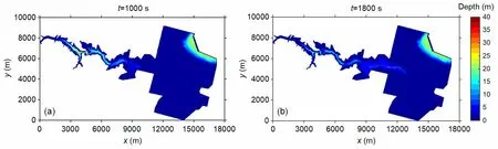
Fig. 10 Malpasset dam break: the flood evolution process

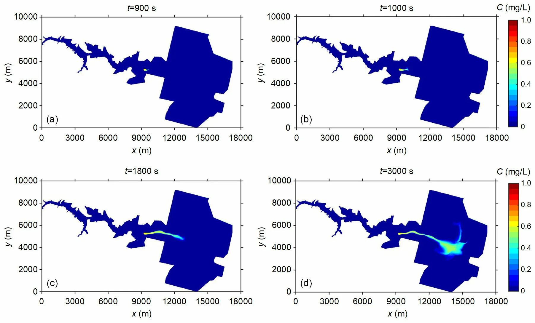
Fig. 11 Results of the solute transport and distribution driven by the flood

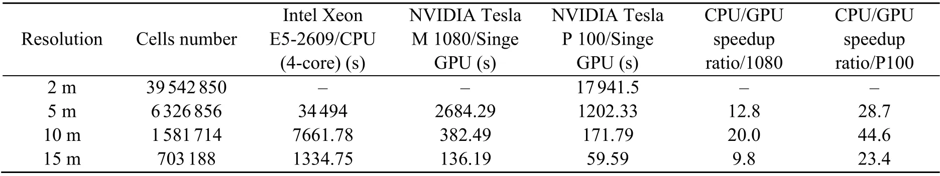
Table 2 Total execution time and speedup ratio by CPU and GPU

The third test example is the advection of solute water driven over three humps by dam-break flood waves. It takes 3.865 s and 13.865 s to complete the 300-s flood event using GPU and CPU computing models, respectively. The fourth case uses different grid resolutions and different hardwares to calculate the flood evolution event. The results show that different GPU models require different times to complete the same event. For different grid resolutions,compared with traditional CPU calculations, GPU computing speed can be increased by 9.8–44.6 times.

The current model is also directly applicable to the practical application of solute transport driven by shallow flows, e.g. the transmission of pollutants in sudden water pollution accidents. This method can be further developed in future work to combine chemical and biological reactions involving the migration of reactive solutes in natural water.

Contributors

Jing-ming HOU and Qiu-hua LIANG developed the numerical model of the GPU-accelerated surface water flow and associated transport. Bao-shan SHI perfected the model and wrote the manuscript. Yu TONG, Yong-de KANG,Zhao-an ZHANG, and Gang-gang BAI helped to organize the manuscript. Xu-jun GAO and Xiao YANG revised and edited the final version. Jing-ming HOU and Bao-shan SHI contributed equally to this work.

Conflict of interest

Jing-ming HOU, Bao-shan SHI, Qiu-hua LIANG, Yu TONG, Yong-de KANG, Zhao-an ZHANG, Gang-gang BAI,Xu-jun GAO, and Xiao YANG declare that they have no conflict of interest.