A novel time-span input neural network for accurate municipal solid waste incineration boiler steam temperature prediction*

Qin-xuan HU, Ji-sheng LONG, Shou-kang WANG, Jun-jie HE,Li BAI, Hai-liang DU, Qun-xing HUANG†‡

1State Key Laboratory of Clean Energy Utilization, Institute of Thermal Engineering, Zhejiang University, Hangzhou 310027, China

2Shanghai SUS Environment Co. Ltd., Shanghai 201703, China

Abstract: A novel time-span input neural network was developed to accurately predict the trend of the main steam temperature of a 750-t/d waste incineration boiler. Its historical operating data were used to retrieve sensitive parameters for the boiler output steam temperature by correlation analysis. Then, the 15 most sensitive parameters with specified time spans were selected as neural network inputs. An external testing set was introduced to objectively evaluate the neural network prediction capability. The results show that, compared with the traditional prediction method, the time-span input framework model can achieve better prediction performance and has a greater capability for generalization. The maximum average prediction error can be controlled below 0.2 °C and 1.5 °C in the next 60 s and 5 min, respectively. In addition, setting a reasonable terminal training threshold can effectively avoid overfitting. An importance analysis of the parameters indicates that the main steam temperature and the average temperature around the high-temperature superheater are the two most important variables of the input parameters; the former affects the overall prediction and the latter affects the long-term prediction performance.

Key words: Waste incineration grate furnace; Neural network; Time-span input; Main steam temperature; Prediction https://doi.org/10.1631/jzus.A2000529 CLC number: TK22

1 Introduction

Large-scale waste incinerators have been built worldwide to deal with municipal solid waste(MSW). By the end of 2018, there were 331 waste incineration plants with a disposal capacity of 365 000 t/d in China (National Bureau of Statistics,2018). Currently, the main types of waste incinerators are grate furnaces and circulating fluidized beds, with grate furnaces forming the majority (Chen and Christensen, 2010). However, several bottleneck problems have restricted the development of this field. First, the vast variance in MSW composition in China results in a large fluctuation in heating value(Zhou et al., 2014), ranging from 2.86 to 9.44 GJ/t(Shapiro-Bengtsen et al., 2020). Second, the large time lag caused by the large capacity of the furnace and the complex coupling effect between various parameters make combustion control and automatic operation difficult to realize. The parameters of the main steam are important monitoring variables,which can be used as an indication of the stability of the operation. Although steam generation can be calculated though the energy balance, the temperature of the steam, especially its pattern of change, is difficult to calculate through traditional methods due to the factors described above. Hence, it is critical to adopt new technologies to predict changes in the main steam temperature for advanced control to avoid instability and overheating (Liukkonen et al., 2011; Han and Zhang, 2012).

Artificial intelligence technology (AI) or artificial neural networks (ANNs) are widely used in complex industrial control processes due to their good nonlinear fitting ability and high robustness (Kalogirou, 2000). They can be used to predict the gasification rate of coal (Chavan et al., 2012) and NOxemissions (Bukovský and Kolovratník, 2012; Bao and Zhang, 2013; Iliyas et al., 2013; Smrekar et al.,2013) to help improve boiler thermal efficiency (Zhao et al., 2010) in pulverized coal boilers. With the rise of the waste incineration industry, studies have also been conducted on the combustion optimization and parameter prediction of waste incinerators. The steam parameters are the focused objects in which different configurations of ANN models are adopted in the prediction of the drum pressure and level (Oko et al.,2015) or the steam temperature, pressure, and mass flow rate (Meher et al., 2015; Shaha et al., 2020). The complex components of waste and its fluctuations in heating value and moisture make understanding the combustion process difficult, which has gained increasing attention in research. Kabugo et al. (2020)reported a neural network-based nonlinear autoregressive model with external input (NN-NARX) for the prediction of the syngas heating value and flue gas temperature of a waste-to-energy boiler. You et al.(2017) conducted a comprehensive comparison of four models, including multilayer perceptron (MLP),adaptive neuro-fuzzy inference system (ANFIS),support vector machine (SVM), and random forest(RF), to consider the online classification of the heating value of solid waste in circulating fluidized bed incinerators; the ANFIS model performed the best. Moreover, the prediction of air pollutants such as CO and SO2in waste incineration has been also investigated through methods such as ANNs or adaptive neuro-fuzzy models (Pai et al., 2015; Norhayati and Rashid, 2018) or by coupling with image processing of the combustion flame (Golgiyaz et al., 2019).

Although satisfactory results have been obtained, previous studies have generally neglected the time lag in large and complex systems by using the simple input-output mapping relationship in the ANN training process, or have focused on prediction of the actual current value rather than on forecasting of the trend, which is of no guiding significance to the operator. This study proposes a neural network model of a time-span input framework that integrates the input data over a time period. The aim is to accurately predict the changing tendency of the main steam temperature in the next 5 min to provide operators with information for a judgment on early adjustment to furnace combustion for stable operation of the system.

2 Object and methods

2.1 Waste incineration grate furnace

The waste incinerator studied in this paper has a daily waste disposal capacity of 750 t/d. Fig. 1 describes the structure of the incineration grate furnace.The grate is divided into three sections, i.e. a drying section, a burning section, and a burnout section, with the primary air system consisting of seven air chambers arranged below it. The primary air volume ranges from 40 000 to 90 000 Nm3/h and is adjusted by controlling the opening of the air chamber. The secondary air volume ranges from 0 to 40 000 Nm3/h.The flue gas temperature in the vertical flue is maintained between 850 °C and 1050 °C to limit the generation of toxic substances. The horizontal flue is arranged with a heat exchanger boiler system. The rated steam temperature is 450 °C, and it generally fluctuates between 430 °C and 455 °C. The main steam pressure varies from 3.85 to 3.97 MPa, and the main steam quantity is 60–80 t/h.

The operating data of each furnace parameter are recorded and stored by the distributed control system(DCS). Operators monitor the parameters through the DCS and flame videos to judge the current operating conditions of the system and to adjust the controlling parameters, such as the air chamber opening and grate speed, to ensure continuous combustion in the furnace and a steady change in the main steam temperature.The longest time period of historical operating data that the DCS can store is one year, with a minimum temporal resolution of 0.5 s.

2.2 Data correlation analysis

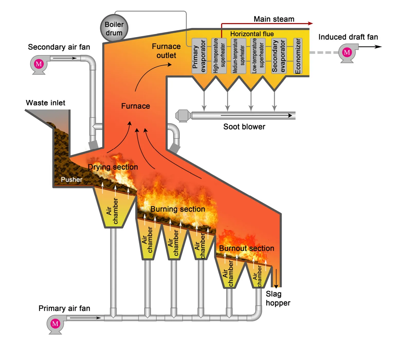
Fig. 1 Structure of the waste incineration grate furnace

The combustion system in the furnace comprises a complex process with multiple parameters, large capacity, non-linearity, and high coupling, where the variables impacting the main steam temperature are distributed in the whole process of combustion and steam-water circulation. According to the heat transfer principle and the operator’s experience, we collected the DCS historical data for 63 variables regarding the temperature and pressure in the furnace,primary and secondary air parameters, grate speed,feed-water, and main steam parameters that may correlate to the main steam temperature. The duration of data collection was 1 week, with a total number of 60 470 records (samples) and a temporal resolution of 10 s.

Some of the 63 variables were imported into the neural network. Due to the exceptionality of engineering, incorrect display or damage to the measuring instrument, it cannot be guaranteed that all 63 variables have effect on the main steam temperature. If some irrelevant variables were added to the input of the network, it may interfere with the training process and increase the training time and computer memory.Hence, filtering of variables with low correlation with the main steam temperature was conducted to simplify the network model.

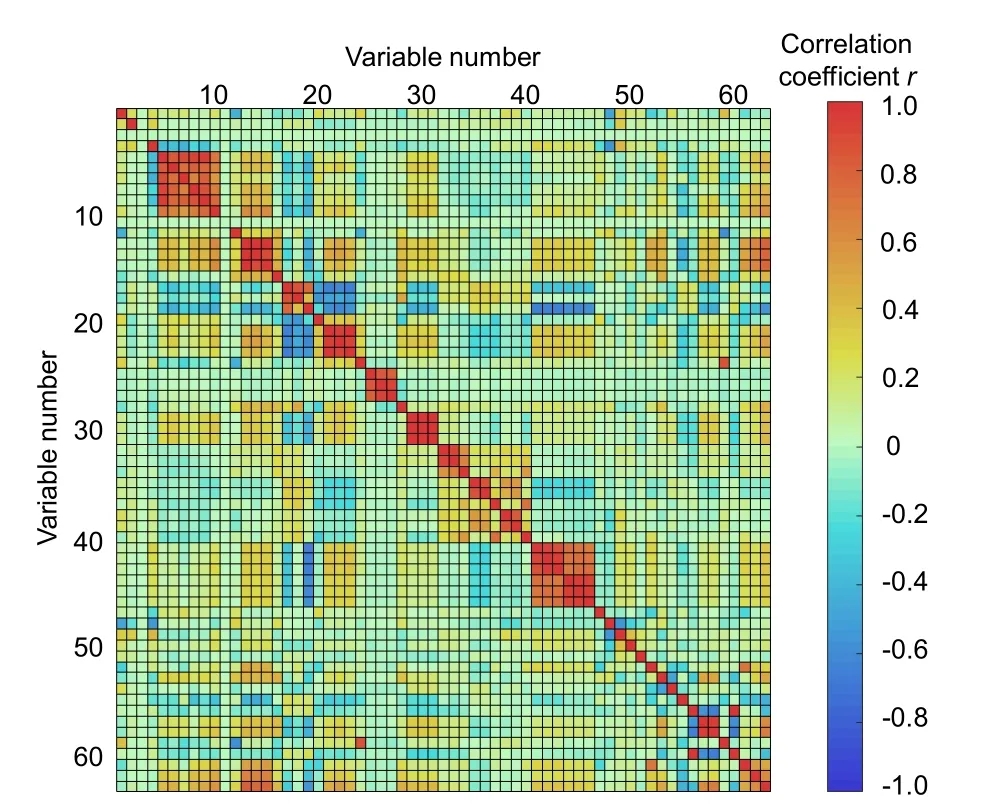
Fig. 2 Two-dimensional thermal matrix of the correlation coefficients of variables

The correlation analysis was carried out in MATLAB, and a 1-d volume of sample data that contained sufficient information on period change was used. Fig. 2 presents the 2D diagonal thermal matrix chart of the correlation coefficients of all 63 variables. The values of the horizontal and vertical coordinates are the indexes of the 1st to 63rd variables, with index No. 61 representing the variable of the main steam temperature (the names of variables are not presented due to space restriction). The scale on the right-hand side represents the value of the correlation coefficient; a positive value represents a positive correlation and a negative value represents a negative correlation. According to the resulting correlation coefficient matrix, variables with an absolute value of the correlation coefficient |r|≥0.3 with the main steam temperature were selected. Combined with experience in engineering practice, 15 variables related to the main steam temperature were selected as input of the neural network. Table 1 exhibits the information and correlation coefficients of these 15 variables, and the historical DCS curves of several representative variables within them are shown in Fig. 3. These variables vary closely with the main steam temperature but there is some time delay between them.

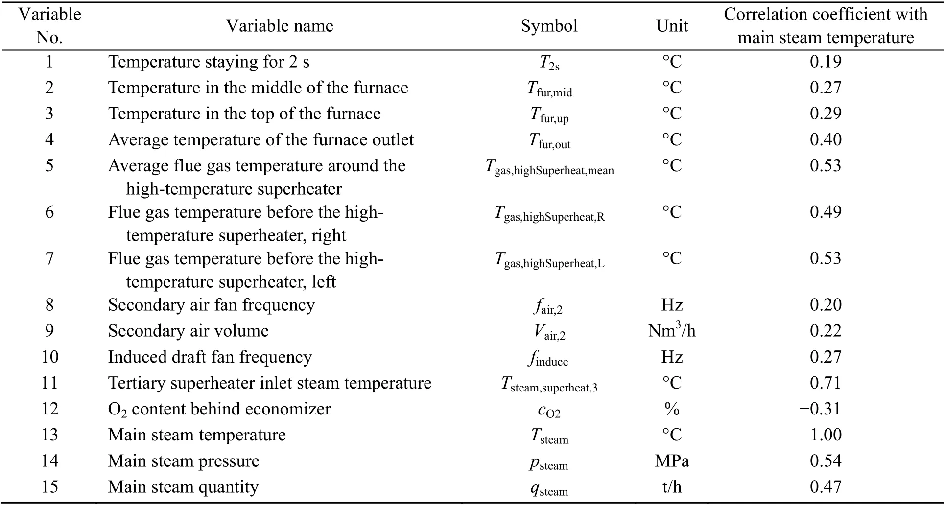
Table 1 Information on variables selected as input for the neural network

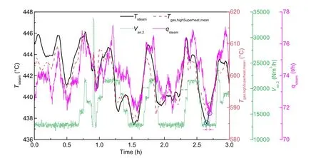
Fig. 3 Time variation of the main steam temperature and of the average flue gas temperature around the high-temperature superheater, secondary air volume, and main steam quantity as recorded by the DCS

2.3 Time-span input framework neural network

A neural network is an algorithm model that simulates the thinking mode of the human brain. It can approximate any nonlinear problem. In this study,the back propagation (BP) neural network with a single hidden layer was adopted, as shown in Fig. 4.The input layer data of the neural network are the DCS data of each selected variable, and the output is the predicted value of the main steam temperature in the future, where each neuron of the output layer represents the predicted value of different future time nodes. The hidden layer of the network contains 10 neurons. Since the output comprehends the predicted values of each time node in the next 5 min, including the result of the current point, and 10 s of predicted step length was adopted, the network output layer has a total of 31 neurons.

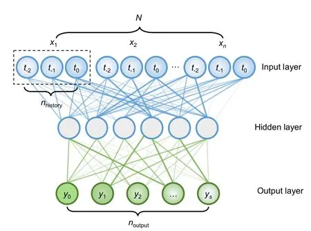
Fig. 4 Structure of the time-span input framework neural network

For the neural network given in Fig. 4, the excitation function of each neuron is described as follows:

whereajandbjare the excitation output value and bias of thejth neuron in the current layer,aiis the output value of theith neuron in the upper layer, andwjiis the connection weight between theith neuron in the upper layer and thejth neuron in the current layer.fis the excitation function of neurons, for which a sigmoid function was adopted. Additional implementation algorithms of the BP neural network are introduced in the literature (Basheer and Hajmeer,2000).

General studies usually take the current value of each variable as the input data of the neural network,which in this paper is called the current time point input framework, to predict the future trend of the target object. Despite the good performance verified in many papers, problems such as insufficient generalization and excessive prediction deviation occur in practical engineering applications. Because of the complexity of the system with a huge capacity and characteristic time lag in industrial furnace combustion, every change in each parameter in the furnace has a certain delay relative to the main steam temperature (Fig. 3), causing untimely adjustment and frequent fluctuation in the operating conditions. As operators in the central control room determine the combustion condition and trend of the main steam temperature based on a period of the DCS historical operating data, this paper proposes a model called the time-span input framework neural network, which integrates the current and time-forward data of each variable in the DCS to predict the future trend of the main steam temperature.

Fig. 5 illustrates the implementation mode of the two types of input frameworks. For each future value prediction ofy1,y2, …,ysat timeti, the current time point input framework only uses a vectorx(i)as the input whereas the time-span input framework uses a matrixX(i)that contains the data at timeti,ti−1, …,ti−das the input, wheredis the number of samples traced forward by taking the current point data as the benchmark. Regarding the time delay problem, the time-span input framework can include this inputoutput time lag information and hence theoretically obtain a better prediction effect.

For a set of time-contiguous samples, the input data of theith sample under the current time point input framework are

wherexj(j=1, 2, …,n) is the current DCS data of each variable. Formsamples, there can beminput vectors.Therefore, the input matrix of the entire sample space can be established

Note that each column of matrixXcorresponds to the entire data of each variable.

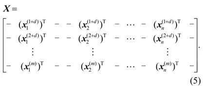
In the time-span input framework, each variable turns into a vector from the original single value. The vector contains the current and time-forward historical data of this variable. All the vectors of variables are combined to form an input matrix. For theith sample, the input matrix is

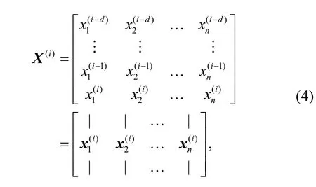
where the number of samples traced forward by taking the current point data as the benchmark (d) under the time-span input framework is the number of periods of DCS data covered except the current point.

In the actual calculation process, the input matrixX(i)is straightened to a whole vector according to the columns to import into the neural network, as shown in Fig. 4. Therefore, formsamples, the input matrix of the sample space can be established as

2.4 Training and testing data sets

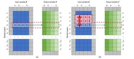
Fig. 5 Input-output mapping relationship of the current time point input framework (a) and the time-span input framework (b)

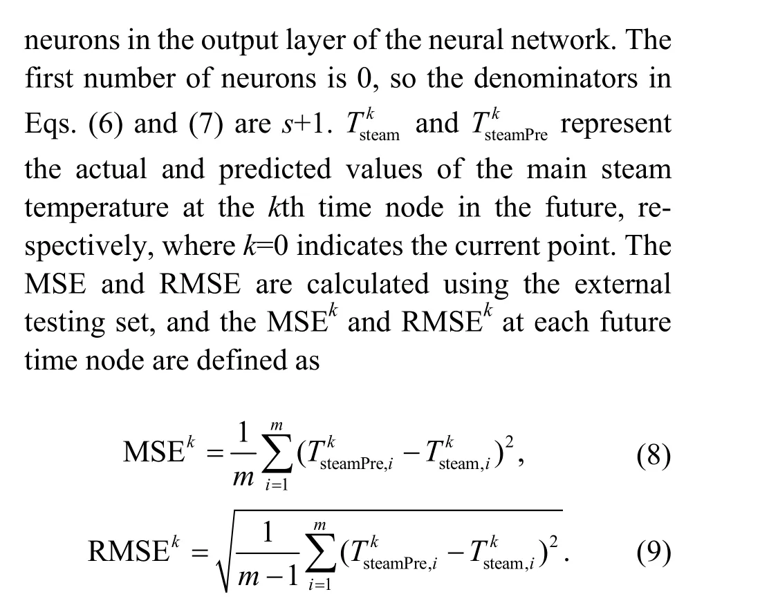
A BP neural network divides the sample data into training, validation, and testing sets before training, and the results of the training set approach the testing set, indicating better generalization ability.Previous trials showed that, despite a close output error of the testing set to the training set calculated through the model, the prediction error was much larger in the actual engineering verification. To more objectively reflect the prediction ability of the model,this paper introduces the concept of an external testing set. In the data disposal process, the samples were divided into two parts: the first part was used for training, testing, and validation of the model, and the second was used for additional testing, and was defined as the external testing set. Fig. 6 shows the time variation of the main steam temperature for the whole period of recorded samples. The first 5 d of samples were randomized (Al Shamisi et al., 2011) and used for training, validation, and testing, and the length ratio of the training, validation, and testing sets was 4׃3׃3. The last 2 d of samples were classified as the external testing set, and the output result was used as the evaluation standard for the model’s performance.It can be observed that the samples of the external testing set cover the whole range of operating conditions, and can be used to evaluate the performance of the model more generally.

3 Results and discussion

The training and computing work was conducted in MATLAB. The default evaluation indicator of the performance of the MATLAB neural network tool is the mean square error (MSE), which may not be intuitive when examining the actual error. To directly compare the actual results with the predicted ones,this study introduces the root mean square error(RMSE) as an evaluation indicator. The MSE or RMSE was used further. The definitions of MSE and RMSE are described as follows:

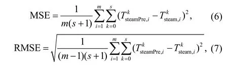
wheremis the sample capacity andsis the number of

Due to the random distribution of initial weights and the use of the stochastic gradient descent method in training, there was a slight difference in the output results of the model after each training. To solve this problem, the model was trained three times after setting the parameters, and the external testing set MSE that deviated greatly from the average was eliminated.The MSE or RMSE obtained through the three trainings were averaged as the performance of the neural network model under the specified parameters.

3.1 Performance comparison between the current time point and time-span input frameworks

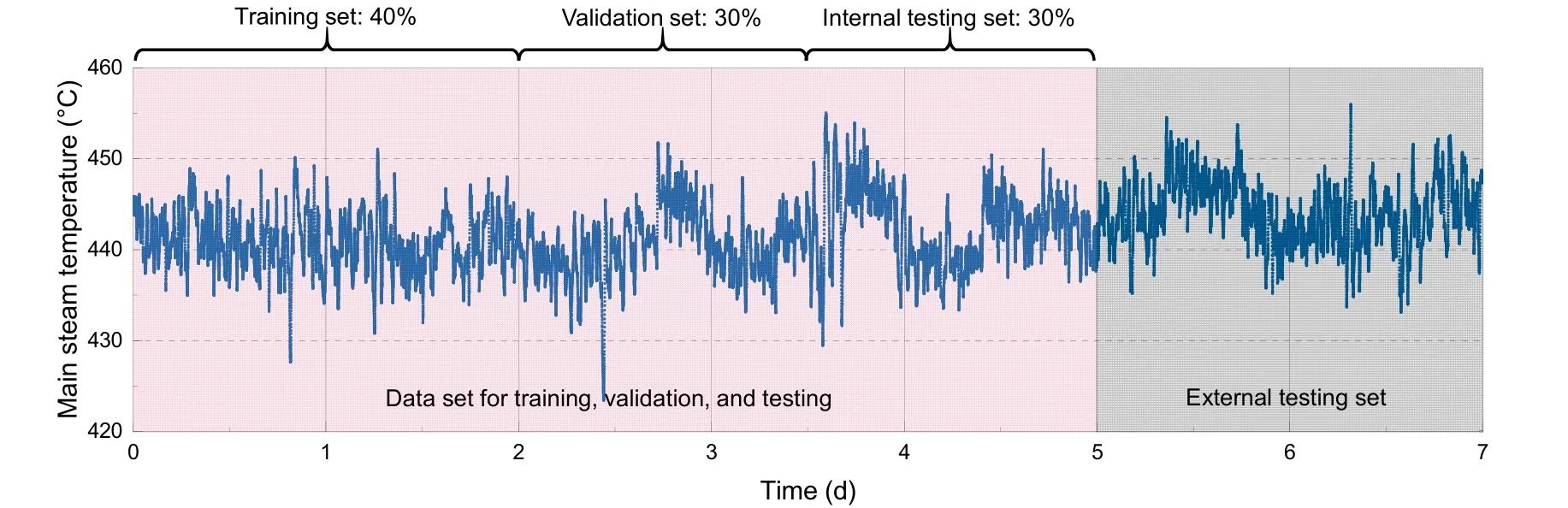
Fig. 6 Time variation of the main steam temperature and sample division

To analyze the prediction performance of the time-span input framework model (referred to as the“time-span model” below), in this study we established the neural network of the current time point input framework (referred to as the “current-time model” below). The two models were combined for analysis. Fig. 7 shows the prediction results of neural networks under different input frameworks. Each diagram displays the actual and predicted main steam temperatures of the current-time model and the time-span model in the next 5 min at different times.The light blue bars show the absolute values of the gradient difference between the curves of the timespan model and the actual value. According to the results shown in Fig. 7 and the calculations, the following conclusions were obtained:

1. According to Eq. (7), the overall root mean square error RMSE of the current-time model is 1.432 °C, and the RMSEof the time-span model is 0.960 °C with an improvement of 33.0%, indicating that the time-span model shows an obvious performance improvement compared with the current-time model.

2. The two models can achieve high prediction accuracy in the short term; the prediction accuracy gradually declines in the long term, which is understandable. As the input variable of the neural network contains the main steam temperature, which inevitably occupies a large weight in the prediction,the prediction results gradually deviate as time progresses due to the uncertainty of the future. However,we find that the prediction accuracy of the time-span model is much higher than that of the current-time model in the long term. A possible explanation is that,in the time-span input framework, the model accumulates the historical variation characteristics of each variable and has the ability to continue the variation inertia for future prediction, thus achieving better prediction.

3. Compared with the current-time model, the predicted values of the time-span model are highly consistent with the actual values in the short term,which is possibly due to the variation characteristics of historical variables contained in the time-span model. Fig. 8 compares the prediction error for each

future time node of the two different models. The RMSE of the current-time model grows quasi-linearly with time, and the time-span model can maintain near-zero prediction error in the first 1 min before the RMSE grows quasi-linearly. In the first 2 min, the prediction accuracy of the time-span model increased by more than 50% compared with the current-time model, and the least improvement was maintained at 22.9% at the 5th minute. The slopes of the RMSEs of the two models were nearly the same in the linear growth part.

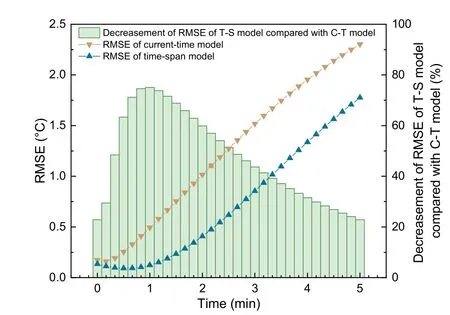
Fig. 8 Prediction RMSEs of two different models in each future time node (the “C-T model” represents the currenttime model, and the “T-S model” represents the time-span model)

It can be concluded that the neural network can achieve good performance when predicting the future trend of the main steam temperature, and the time-span model has a better prediction capability than the current-time model. In some cases, when the prediction results of the current-time model have significantly deviated from the actual value, the time-span model can still trace the actual trend well(Figs. 7a, 7d, 7e, and 7j) in the short term (first 1 min)and even the long term (Figs. 7b, 7j, 7k, and 7p).Although it can achieve considerably high prediction accuracy, it requires more training time than the current-time model.

The trained model can achieve real-time computing. Using an Intel I7 CPU-based PC, the time consumed for a single calculation of the prediction using the time-span model is approximately 45 ms,providing the possibility for real-time online prediction of the system, and the prediction can be updated through high-frequency calculation to constantly correct the error.

3.2 Analysis of the time-span input framework neural network

The time-span input framework neural network achieves better prediction accuracy and generalization ability at the expense of geometric growth of the occupied training time and computational memory attributed to the multiple increases in input data.Hence, the problem of “cost performance” should be considered. This section focuses on the influences of the parameters and structure of the time-span neural network analyzed above on the prediction result.Since the MSE is the default performance indicator in the MATLAB neural network fitting tool, most of this section uses the MSE for analysis.

3.2.1 Terminal training threshold

The generalization ability of neural networks is one of the most popular issues in this field. A high prediction precision means a low generalization ability (Tzafestas et al., 1996). Hence, a balance between them should be considered. The BP neural network has a good generalization ability due to its structural characteristics. The Bayesian regularization model and time-span input framework adopted in this study also facilitate the generalization ability. However,there is still error in the long-term prediction; furthermore, in some cases, the predicted changing tendency directly deviates from the actual value(Figs. 7d, 7f, and 7l).

Controlling the terminal conditions of training is a method to prevent overfitting of neural networks(Srivastava et al., 2014). The default terminal condition of the training in this study is the minimum training gradient falling below 0.1 without the limit of iteration. Under these circumstances, the MSE of the network will continue to decrease until the model is trained to the extreme. In this part, the terminal MSE threshold of training is set. When the MSE of the training set falls below the threshold, the training process is terminated, and the generalization ability of the network under different terminal training thresholds is analyzed. To evaluate whether the model is overfitting, new sample data that have no intersection with the training process, namely, the “external testing set”, are adopted for verification.

After several attempts, the final terminal MSE thresholds of training set were set to 0.46, 0.48, 0.50,0.52, and 0.54. Fig. 9 shows the MSE of the training set, internal testing set, and external testing set under each terminal training threshold, in which “non”stands for no limit. The error bars represent the ranges of three training results under the same parameters of the network. As it can be seen, the MSE of the external testing set decreases with the increase in the terminal training MSE threshold and is basically in a stable state in cases of terminal training MSE greater than 0.48. The maximum ratio of training set MSE to external testing set MSE was 66.8% at the terminal training threshold MSE of 0.54, which indicates a generalization ability of 66.8%. If the terminal threshold of training is not limited, the model does result in overfitting, and the MSE difference of the three trainings of the external testing set reaches 0.162 (°C)2, 245.5% greater than the MSE difference of 0.07 (°C)2at the terminal training MSE of 0.5,leading to uncertainty in the model training. One explanation is that the overtrained model may fall into different local minimum regions, resulting in different output performances.

Fig. 9 Prediction results of the model under different terminal training thresholds

An interesting phenomenon is shown in Fig. 9:when the terminal training MSE is 0.46, the internal testing set MSE is less than that when the terminal training MSE is 0.52 whereas the result is quite the opposite for the external testing set. Thus, it is not sufficient to verify the generalization performance using only the testing set assigned by the neural network itself, and an external testing set is also needed.

3.2.2 Time span of the input data

This section discusses the influence of the time span of the input data on the performance of the neural network model and the cost of training.

According to the conclusion obtained in Section 3.2.1, the terminal training threshold of the model was set at 0.5 to adapt to the training margin of different time spans of input data. The time span of the input was set as 20 s, 40 s, …, 200 s. Fig. 10 shows the results, and the error bars represent the ranges of three training results under the same parameters of the network. With the increase in the time span, the external testing set MSE generally presents a downward trend, meaning that the prediction accuracy continues to improve. When the time span is longer than 80 s,the external testing set MSE fluctuates in equilibrium,with an average reduction of 31.3% compared with that in the cases of time span less than 40 s. The generalization ability, that is, the ratio of the training set MSE to the external testing set MSE, is approximately 60% for the cases of time span more than 80 s.In the cases of 20-s and 40-s time spans, the training set MSE did not drop to the threshold of 0.5, which means both reach the limit of their training, leading to the significant deviation of the external testing set MSE from the others.

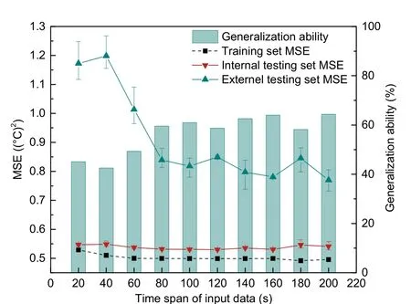
Fig. 10 Performance of the model under different time spans of input data

The time-span input framework neural network can achieve good prediction performance. However,it is costly to adopt this framework, as the volume of input data is much larger than that of the current-time model. Fig. 11 shows the relationship between different time spans of input data and the training time of a single iteration of the neural network. With the increased volume of input data, the single iteration time undergoes exponential growth. Taking the 16-core Intel i7 CPU PC as an example, when the time span increases to 200 s, a single iteration time takes approximately 13 min, which is disadvantageous no matter for the scientific research or for the engineering debugging.

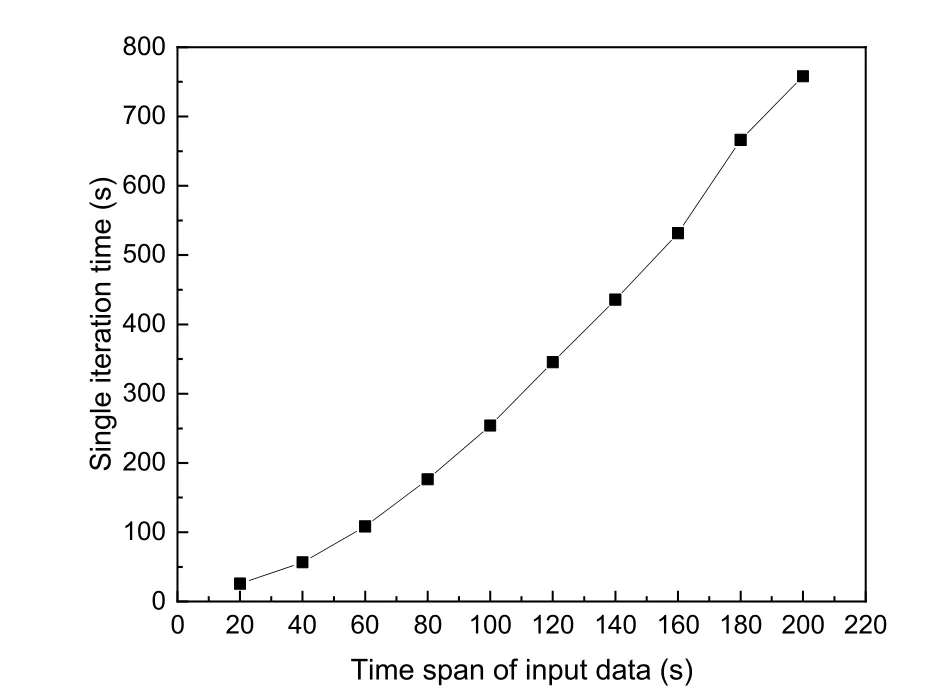
Fig. 11 Relationship between the time span of input data and single iteration time of the neural network

Fig. 12 shows the average numbers of iterations and training times of the model under different time spans of input data. On the whole, the number of iterations decreases sharply with increasing time span and finally reaches a stable state. However, according to the conclusion from Fig. 11 that the time for a single iteration increases with increasing time span,the overall training time first presents a downward trend and then increases. In the cases of 20-s and 40-s time spans, the time consumed for three trainings varies widely, with the standard deviation reaching 7776 s and 5425 s, respectively, due to overtraining,which is unfavorable to the qualitative analysis of the model.

The above analysis is based on the overall prediction error of the output. For the tendency prediction problem, it is necessary to focus on the results of each time node to evaluate the short-term and long-term performances of the model. Fig. 13 shows the prediction errors at each future time node of the models with different time spans of input data, where the time span of input data equal to 0 s represents the current-time model. The RMSEkof the external testing set was applied to compare the prediction errors intuitively.

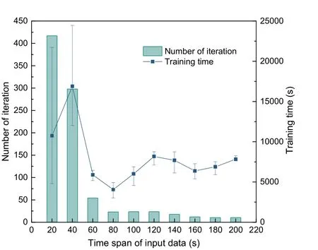
Fig. 12 Training cost of the model with different time spans of input data

As expected, as time progressed, the prediction error of each case increased gradually. However, it is worth noting that the average RMSE of the model with only a 20-s time span of input was significantly reduced by 28.2% compared with the current-time model. In the first 1 min, the prediction error of all time-span models reached an ultrahigh precision of 0.2 °C, which is markedly distinguished from the current-time model in the trend of time-progressed prediction error. The maximum prediction error of the best-performing time-span model from Fig. 13 at the 5th minute can be reduced to nearly 1.5 °C. The prediction RMSEkwas basically the same when the time span of the input data was greater than or equal to 80 s, which is consistent with the results shown in Fig. 10.

3.3 Importance of parameters

A neural network is similar to a black box; it can fit the results well but cannot provide explanatory insight (Olden and Jackson, 2002). In practical applications, people pay more attention to the mapping relationships between input and output variables.Therefore, it would be of great value to engineering and network optimization if the influence of each input on the output could be learned.

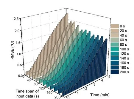
Fig. 13 Prediction RMSEs of each future time node of the model with different time spans of input data

Importance analysis is an effective way to study the influence of input variables. The relative importance of a variable refers to how much the existence of the variable affects the output. There are many ways to analyze the importance of input variables of a neural network. One effective method is to remove a whole variable and recalculate how much the output MSE changed, that is, the change of the mean square error (COM). The concrete implementation of this method has been described (Sung, 1998). This study makes some modifications to the method. First, the RMSE is used instead of the MSE to calculate the change in root mean square error (COR) (Tóth et al.,2017) so that the scope of change can be detected intuitively. The definition of the COR is

wherekis thekth future time node andnis the removal of thenth input variable. Second, the original paper retrained the neural network after removing a variable and then observed the change in MSE. As the neural network will conduct random weight initialization before each training, different initialized weights of the network will produce a slight difference in the output results after training. Furthermore,due to the adaptive ability of the weights of neurons,the impact of the eliminated variable on the results may be compensated by adjustment of the weights of other variables. To avoid the interference of the above factors, we recalculated the existing model according to Eq. (1) after setting the weights of each neuronwjiin the hidden layer connecting the specified input variableito zero instead of retraining the model.

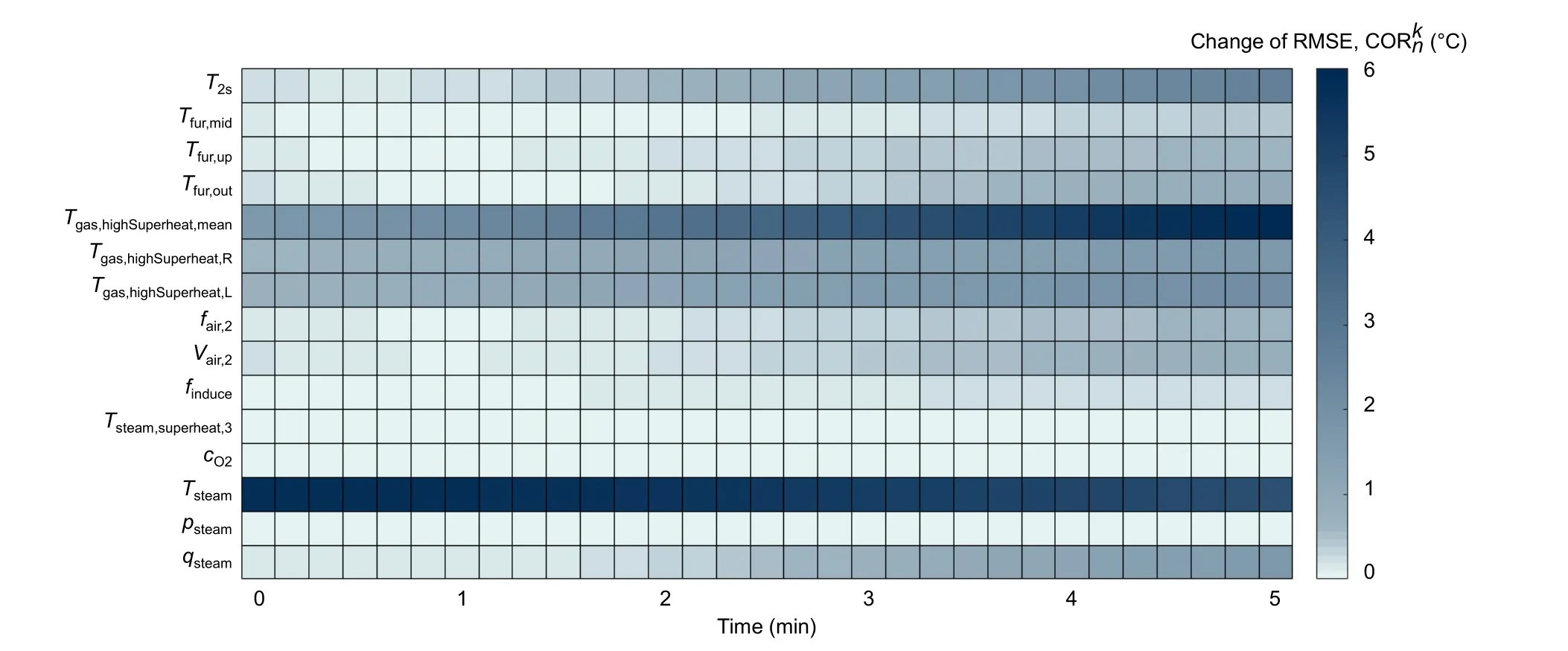
Fig. 14 CORs of prediction of the main steam temperature at each future time node after removing different variables

According to the results analyzed in Section 3.2 and considering the generalization and time cost for training, the final terminal training threshold was set as 0.5 and the time span of the input data was 160 s.Fig. 14 shows the COR of the main steam temperature at each future time node after the removal of different variables. The darker area in the figure indicates a higher value of COR and greater importance of the variable. As expected, the main steam temperatureTsteamhas the greatest impact on itself in the future due to the baseline provided for prediction. WhenTsteamwas removed from the model, the prediction error increased by a maximum of nearly 6 °C. The second most important variable is the average flue gas temperature around the high-temperature superheaterTgas,highSuperheat,mean, and the maximum variation of the prediction error reached 6 °C. The comparatively important variables are the temperatures in the furnace and horizontal flue, the main steam quantity,the secondary air frequency, and air volume; the residual variables are of low or no importance to the output.

Fig. 14 shows that the variables generally present increasing importance in the long-term prediction; the most obvious was theTgas,highSuperheat,mean,with an increase in the COR by 4.35 °C from the beginning to the end. Due to the uncertainty of the far future, if a variable was missing in the model, the calculated error would be larger in the long-term prediction. However, the variableTsteampresents the opposite characteristic, with COR decreasing by 1.25 °C from the beginning to the end. This is understandable. The variableTsteamcomprises a large weight of the prediction of the main steam temperature and omitting the temperature will cause a fundamental deviation of the short-term prediction. For long-term prediction, this large deviation may be gradually corrected by other variables as time progresses. Despite the importance ofTsteampresenting a decreasing trend over time, the COR ofTsteamat the 5th minute was still maintained at 4.52 °C, meaning thatTsteamwas not less significant for long-term prediction.

According to the importance analysis of the variables, there are some control measures for the main steam temperature. It is suggested that the average temperature around the high-temperature superheater is the focus. When the predicted trend of the main steam temperature is rising, it can be regulated by adjusting the secondary air volume to decrease the temperature around the high-temperature superheater or by increasing the main steam quantity to increase the heat capacity of the boiler.

4 Conclusions

This work studied a neural network with a time-span input framework, which was used to predict the trend of the main steam temperature of a 750-t/d waste incineration grate furnace over the next 5 min. The prediction result can be used to optimize the combustion in the furnace to avoid system fluctuation and overheating of the steam. First, parameters with relatively high correlation with the main steam temperature are extracted according to correlation analysis, and historical DCS data of selected variables are used to train the neural network. An external testing set that has never participated in the network training process is introduced to objectively test the performance of the network. In this paper we comparatively analyzed the current time point input framework model and the time-span input framework model. The results show that the time-span model has a better prediction performance and generalization ability, with a prediction error for the first 60 s of the future reaching near-zero, and the maximum prediction error being reduced almost to 1.5 °C. This paper also analyzed the impact of the terminal training threshold and time span of the input data on the performance and training cost of the neural network and discussed the causes of overfitting in the network.The importance analysis of variables shows that the main steam temperature has the greatest impact on its trend prediction, and the average flue gas temperature around the high-temperature superheater deeply influences the long-term prediction. The trained model can instantaneously calculate the prediction results based on DCS historical data, providing the possibility of real-time online prediction.

Contributors

Qin-xuan HU designed the research and wrote the first draft of the manuscript. Ji-sheng LONG, Li BAI, and Hai-liang DU provided the data and studied the structure of the furnace.Shou-kang WANG and Jun-jie HE helped to process the corresponding data. Qun-xing HUANG revised and edited the final version.

Conflict of interest

Qin-xuan HU, Ji-sheng LONG, Shou-kang WANG,Jun-jie HE, Li BAI, Hai-liang DU, and Qun-xing HUANG declare that they have no conflict of interest.