Subgroup analysis for multi-response regression

Wu Jie, Zhou Jia*, Zheng Zemin*

1. International Institute of Finance, University of Science and Technology of China, Hefei 230601, China;2. School of Management, University of Science and Technology of China, Hefei 230026, China

Abstract: Correctly identifying the subgroups in a heterogeneous population has gained increasing popularity in modern big data applications since studying the heterogeneous effect can eliminate the impact of individual differences and make the estimation results more accurate. Despite the fast growing literature, most existing methods mainly focus on the heterogeneous univariate regression and how to precisely identify subgroups in face of multiple responses remains unclear. Here, we develop a new methodology for heterogeneous multi-response regression via a concave pairwise fusion approach, which estimates the coefficient matrix and identifies the subgroup structure jointly. Besides, we provide theoretical guarantees for the proposed methodology by establishing the estimation consistency. Our numerical studies demonstrate the effectiveness of the proposed method.

Keywords: multi-response regression; subgroup analysis; concave penalties; ADMM algorithm

1 Introduction

Rapid developments in technology have brought in massive data sets in various fields ranging from health, genomics and molecular biology, among others. In these applications, identifying subgroups from a heterogeneous population is of great importance since it reveals domain knowledge behind the data. For example, experimental studies have shown that the relative efficacy of antiretroviral drugs for treating human immunodefciency virus infection sometimes depends on baseline viral load and CD4 count[1]. Similarly, in the study of clinical trials, it has been increasingly recognized that some subgroup of patients can benefit from a treatment or suffer from an adverse effect much more than the others[2]. Therefore, recovering the heterogeneous effects has gained increasing popularity in data analyses.

A popular method for analyzing data from a heterogeneous population is to view data as coming from a mixture of subgroups, where their own sets of parameter values should be estimated using finite mixture model analysis[2-4]. However, these mixture model-based approaches need to specify the underlying distribution of data and the number of mixed components in the population, which are often difficult to satisfy in real applications. By contrast, several other methods consider the problem of exploring homogeneous effects of the covariates by assuming that the true coefficients are divided into a few clusters with common values. For example, Guo et al.[5]proposed using a pairwiseL1fusion penalty for identifying variables in the context of Gaussian model-based cluster analysis. Chi and Lange[6]proposed to multiply nonnegative weights to theL1norms to reduce the bias. The major advantage of such methods is that they can detect and identify heterogeneous subgroups without knowledge of a priori classification. But theL1penalty generates large biases in the estimates in each iteration of the algorithm, thus leading to incorrect conclusions. Furthermore, Wang et al.[7]applied a two-stage multiple change point detection method to determine the subgroups and estimated the regression parameters. Similarly, Li et al.[8]proposed an estimation procedure combining the likelihood method and the change point detection with the binary segmentation algorithm. Despite a well estimation accuracy of these two methods, it is unclear how to verify the theoretical properties.

To address these issues, Ma and Huang[9]proposes a new method in which the heterogeneity can be modeled through subject-specifc intercepts in regression and can be implemented via a concave pairwise fusion penalized least squares without a priori knowledge of classification, thus more desirable for identifying subgroups. But this method is only applicable to heterogeneous univariate regression, and how to deal with heterogeneous multi-response regression is still unknown, which restricts the efficiency of the method. Although there exist many literature focusing on multi-response regression[10-15], which represent the dependency between the multiple outcomes and the same set of predictors, these method are no longer valid in face of the problem related to the data from a heterogeneous population.

In this article, we develop a new methodology for heterogeneous multi-response regression, which estimates the coefficient matrix and identifies the subgroup structure jointly. The proposed estimator utilizes the idea proposed By Ma and Huang[9], that is, applying the concave pairwise fusion penalized least squares, but extends the univariate heterogeneous regression to a multiple one. The major contributions of this paper are twofold. First, we develop a new method for heterogeneous multi-response regression, which automatically divides the observations into subgroups without a prior knowledge of classification. Second, we provide theoretical guarantees for the proposed method by establishing estimation consistency and derive the convergence properties of the algorithm.

The remainder of this paper is organized as follows. Section 2 presents the model setting and our new methodology. Theoretical properties of the proposed method are established in Section 3. We provide numerical studies in Section 4. Section 5 concludes with extensions and possible future work. The proofs and additional technical details are provided in the Appendix.

2 Subgroup analysis for multi-response regression via concave pairwise fusion

2.1 Model setting

Consider the following heterogeneous multi-response regression model

Y=XB+C+E

(1)

whereY=(y1,…,yn)Tis ann×qresponse matrix,X=(x1,…,xn)Tis ann×pcovariate matrix,Bis ap×qcoefficient matrix,C=(c1,…,cn)Tis ann×qintercept matrix andE=(e1,…,en)Tis ann×qrandom error matrix. One interesting application of the model is precision medicine where the responses vector could be several phenotypes associated with some disease and predictors are a set of observed characters such as gender, sex, age and so on. After adjusting for the effects of the covariates, the distribution of the response is still heterogeneous. It means that the heterogeneity can be the result of unobserved latent factors which can be modeled through the subject-specifc intercept vectors, similar as that in Ref.[9]. Specifically, the heterogeneous structure can be modeled as follows

whereα=(α1,…,αK)Tis aK×qmatrix andαkis the common vector for theci’s in thekth subgroup, andWis ann×K(latent) indicator matrix in whichwik=1 forciinkth group andwik=0 otherwise. Substituting this into model (1) yields the final multi-response heterogeneous model:

Y=XB+Wα+E

(2)

Letψ=(ψ1,…,ψK) be a partition of {1,…,n}. Without loss of generality, we assume thatY=(y1,…,yn)Tare fromKdifferent groups withK≥1 and the data from the same group have the same intercept vectorαi, i.e.ci=αkfor alli∈ψk.

Although we adopt a similar estimation idea proposed in Ref.[9], how to apply the method under multi-response regression model here is a nontrivial task even if it is conceptually straightforward. Our goal is to correctly estimateK, identify the subgroups of outcomes and accurately estimate the regression coefficient matrixB.

2.2 Algorithm

Consider that the heterogeneous treatment effects are characterized by the intercept matrix, to estimate the unknown parameter matrixBand intercept matrixCjointly, a direct idea is to solve the following penalized least square problem

(3)

wherepr(·,λ) is a penalty function indexed by the tuning parameterλ≥0, indicating the amount of penalization. By minimizing the objective function, the penalty functionpλ(.) shrinks some ‖ci-cj‖2to 0, thus automatically dividing the samples into different subgroups. Givenλ>0, the estimates of the coefficient matrices are defined as

(4)

However, the penalty function in the above optimization problem (3) is not separable inci. We then reformulate the problem as follows by resorting toδij=ci-cj,

s.t.ci-cj-δij=0

(5)

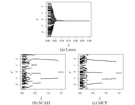
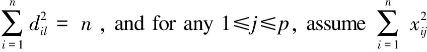
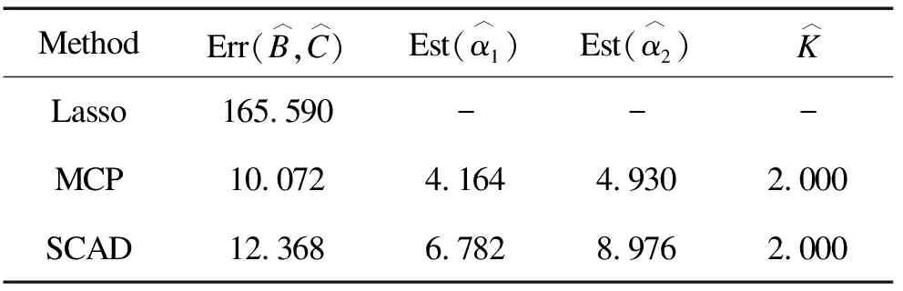
whereδ={δij,i

L(C,B,δ,v)=L0{C,B,δ}+

(6)

(7)

(8)

(9)

Sinceδmandvmare fixed in the first step, the problem (7) can be simplified as

whereCnis a constant independent of (C,B). Through some algebra, we rewritef(C,B) as

(10)

whereA={(ei-ej),i

(11)

Bm+1=(XTX)-1XT(Y-Cm+1)

(12)

whereQX=X(XTX)-1XTdenotes the orthogonal projection matrix onto the range ofXandIndenotes the identity matrix. In the second step, we discard the terms independent ofδand minimize the problem (8) as follows

(13)

for theL1penalty[16]or

(14)

for the MCP[17]withγ>1/υor

(15)

for the SCAD penalty[18]withγ>1/υ+1. At last, the update ofvijis given in (9). We terminate the algorithm when the stopping criterion met. To be specific, we stop the algorithm oncerm+1=ACm+1-δm+1is close to zero such that ‖rm+1‖F

The efficiency of subgroups identification via our method can be seen from a simple simulation example summarized in Figure 1, where the data are generated similarly as in Section 4 except that each row ofC*is generated i.i.d. from three different vectorsα1,α2,α3with equal probabilities. That is,

Figure 1. Solution paths for against λ for data in Section 2.

Figure 2. Solution paths for against λ for data in Section 4.

withα1=(2,…, 2),α2=(0,…, 0) andα3=(-2,…, -2). It is clear that the estimators using concave penalties MCP and SCAD can accurately identify the subgroups while convex penalty Lasso merge to one value quickly due to the overshrinkage of theL1penalty.

3 Theoretical properties

In this section, we study the theoretical properties of the proposed estimator. Specifically, we provide sufficient conditions under which there exists a local minimizer of the objective function equal to the oracle least squares estimator with a priori knowledge of the true groups with high probability. We also derive the lower bound of the minimum difference of the coefficients between subgroups to estimate the subgroup-specific treatment effects.

3.1 Notation and conditions

Let Mψ={C∈n×q} :ci=cj, fori,j∈ψk, 1≤k≤K. For eachC∈Mψ, It can be written asC=Wα, whereα=(α1,…,αK)Tandαkis aq-dimension vector of thekth subgroup fork=1,…,K. Simple calculation shows

WTW=diag(|ψ1|,…,|ψK|),

ρ(t)=λ-1Pγ(t,λ).

We make the following basic assumptions.

Condition 3.1For some constanta>0, the functionρ(t) is constant oncet≥aλ. It is symmetric, non-decreasing and concave on [0,∞). In addition,ρ′(t) exists and is continuous except for a finite number values oft,ρ′(0+)=1 andρ(0)=0.

Condition 3.2The noise vector=(1,…,n)Thas sub-Gaussian tails such thatP(|aT|>‖a‖2x)≤2exp(-c1x2) for any vectora∈nandx>0, where 0

Conditions 3.1 puts a mild assumption on the penalties and it is obviously that the concave penalties such as MCP and SCAD satisfy it. Condition 3.2 is standard in the penalized regression in high-dimensional settings. Condition 3.3 imposes conditions on the eigenvalues of the population covariance matrixUTU. Note thatλmin(WTW)=|ψmin|. By assumingλmin(XTX)=Cn, we have

λmin|(W,X)T(W,X)|≤ min (|ψmin|,Cn).

The equality holds whenWTX=0. Hence, we assumeλmin[(W,X)T(W,X) ]≥C1|ψmin| for some constant 0

Before giving the detail theorem, we also need to introduce a new definition called oracle estimators, which are not real estimators but theoretical constructions useful for stating the properties of the proposed estimator. When the true group membershipsψ1,…,ψKare known, the oracle estimators forBandCare solved by

and correspondingly, the oracle estimators for the common intercept vectorαand the coefficient matrixBare given by

(16)

Letα0=(α1,…,αK)T∈K×q, whereis the underlying common intercept vector for the groupψk. LetB0be the underlying regression coefficient matrix. Now we are ready to show the main results.

(17)

and

where

(18)

Remark 3.1ForK≤2, let

be the minimal difference of the common values between two groups.

4 Simulation studies

In this section, we use simulated data to investigate the finite sample performance of the proposed method via two concave penalties, the smoothly clipped absolute deviation (SCAD), the minimax concave penalty (MCP) and one convex penalty (Lasso), in comparison with the classic method reduced rank regression (RRR). Among them, MCP, SCAD and Lasso have two tuning parameters including rank and sparse parameter, which are selected jointly by BIC. By contrast, RRR only has one tuning parameter rank, which is also tuned by BIC for fair comparison of all methods.

Table 1. The sample mean and standard deviation (S.D.) of estimators (1×102). n=100, p=12, K=2.

In view of the results in Table 1, it is clear that our proposed estimators using concave penalties MCP and SCAD enjoy higher accuracy than utilizing convex penalty Lasso or classic method RRR which does not consider heterogeneous effects. Although similar to MCP and SCAD, Lasso consider a heterogeneous effects, but it tends to over-shrink large coefficients, thus leads to biased estimates and unable to correctly recover subgroups. In view of the heterogeneous estimation results in Table 1, both MCP and SCAD can identify the subgroups while RRR and Lasso have worse performance than the MCP and SCAD penalties. Specifically, the heterogeneity related measures do not apply to Lasso and RRR since they do not recover the latent subgroup structures. From another point of view, Lasso and RRR can not recover and utilize the heterogeneous structure, which in turn lowers its estimation and prediction accuracies about coefficient matricesB*andC*.

5 Application to the yeast cell cycle data set

In this section, we will analyze the yeast cell cycle data set originally studied in Ref.[19]. This data set consists of 524 yeast genes, the RNA transcript levels (X) of which can be regulated by transition factors (TF) within the eukaryotic cell cycle. Specifically, 21 of the TFs were experimentally confirmed related to cell cycle process. It covers approximately two cell cycle periods with measurements at 7 min intervals for 119 min with a total of 18 time points (Y). Similar to Ref.[13], we considered the multi-response regression model to estimate the association coefficient matrix between the transition factors and the cell cycle gene expression data. Then we artificially added the intercept matrixCsimilarly as in Section 4 to generate subgroup structure, whereC=(c1,…,cn)T. Each row ofCis generated i.i.d. from from the distribution:

P(ci=α1)=P(ci=α2)=1/2

withα1=(2,…, 2) andα2=(0,…, 0). Based on the processed data set, we identify the subgroups via Lasso, SCAD and MCP. Since the underlying model is unknown, we report the surrogate estimation error

with the true covariate matrixXto evaluate the estimation accuracy of the regression coefficient matrix. The results for our proposed method are summarized in Table 2. In view of the results, MCP achieved the highest accuracy in view of the estimation errors. Both MCP and SCAD can successfully identify the true subgroups.

Table 2. The performance measures of estimators (1×102).

6 Conclusions

In this paper, we have extended the method for heterogeneous univariate-response regression to multi-response regression, which recovers regression coefficient matrix and latent heterogeneous factors by concave pairwise fusion penalties. Numerical studies demonstrate the statistical accuracy of the proposed method. Our estimation procedure may be extended to deal with data containing censoring, measurement errors and outliers or more general model settings such as the generalized linear model, which will be interesting topics for future research.

Acknowledgments

This work is supported by National Natural Science Foundation of China (Nos. 72071187, 11671374, 71731010, and 71921001), and Fundamental Research Funds for the Central Universities (Nos. WK3470000017 and WK2040000027).

Conflictofinterest

The authors declare no conflict of interest.

Authorinformation

WuJieis currently a PhD candidate at School of Management, University of Science and Technology of China. She received her BS degree from Anhui University of Technology in 2017. Her research mainly focuses on high dimensional variable selection, classification.

Zhoujia(corresponding author) is currently a PhD candidate at School of Management, University of Science and Technology of China. She received her BS degree from Anhui University of Finance and Economics in 2016. Her research mainly focuses on high dimensional variable selection and statistic inference.

ZhengZemin(corresponding author) is Full Professor at Department of Management, University of Science and Technology of China (USTC). He received his BS degree from USTC in 2010 and PhD degree from University of Southern California in 2015. Afterwards, he is working in Department of Management， USTC. His research interests include high dimensional statistical inference and big data problems. He has published some high-level articles in top journals of Statistics, includingJournalofRoyalStatisticalSocietySeriesB,TheAnnalsofStatistics,OperationsResearch, andJournalofMachineLearningResearch. In addition, he has also presided over several scientific research projects, including the Youth Project of the National Natural Foundation of China (NSFC), General Projects of the NSFC.