A hybrid HWENO-based method of lines transpose approach for Vlasov simulations

Wang Kaipeng, Jiang Yan, Zhang Mengping

School of Mathematical Sciences, University of Science and Technology of China, Hefei 230026, China

Abstract: A new type hybrid Hermite weighted essentially non-oscillatory (HWENO) schemes in the implicit method of lines transpose (MOLT) framework is designed for solving one-dimensional linear transport equations and further applied to the Vlasov-Poisson (VP) simulations via dimensional splitting. Compared with the WENO-based MOLT method given in J. Comput. Phys. [2016, 327: 337-367], the new proposed hybrid HWENO-based MOLT scheme has two advantages. The first is the HWENO schemes using the stencils narrower than those of the WENO schemes with the same order of accuracy. The second is that the schemes can adapt between the linear scheme and the HWENO scheme automatically. In summary, the hybrid HWENO scheme keeps the simplicity and robustness of the simple WENO scheme, while it has higher efficiency with less numerical errors in smooth regions and less computational costs as well. Benchmark examples are given to demonstrate the robustness and good performance of the proposed scheme.

Keywords: method of lines transpose; implicit time discretization; HWENO methodology; hybrid scheme; Vlasov-Poisson system

1 Introduction

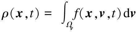
In this paper, we develop efficient numerical solvers for the Vlasov-Poisson (VP) system, which is considered a fundamental model in plasma physics describing the dynamics of charged particles due to the self-consistent electric force. The VP system is given as follows:

(1a)

(1b)

Besides the famous “curse of dimensionality”, the main challenge of VP system is that the solution may develop filamentation solution structures under the long-range forces. Examples will be shown later. Consequently, numerical scheme needs careful design such that it can effectively capture filamentation structures without producing spurious oscillations.

There exist a large amount of successful VP solvers in the literature, such as Eulerian type approaches[1-4], and the semi-Lagrangian approach[5-17], and the Lagrangian methods, which including the particle-in-cell (PIC) method[18-20]and Lagrangian particle methods[21,22]. However, each method has its own limitations. For example, Eulerian approaches are suffering from the CFL time step restriction; general boundary conditions are difficult to handle in a semi-Lagrangian setting; and the Lagrangian methods are known to suffer from low order sampling noise. Many of these existing methods are in the method of line (MOL) framework, meaning that the spatial variable is first discretized, then the numerical solution is updated in time by coupling a suitable time integrator.

Recently, an alternative approach to advance the solution called the method of line transpose (MOLT) is well designed to solve the VP system[23]. This method is also known as the Rothe’s method or transversal method of lines in the literature[24,25]. In this framework, the discretization is first carried out for temporal variable, resulting in a boundary value problem (BVP) at the discrete time levels. Each BVP can be inverted analytically in an integral formulation based on a kernel function and then the numerical solution is updated accordingly. A notable advantage of such a scheme is that, even though it is implicit in time, we do not need to explicitly solve a linear system, while the BVP is inverted analytically in an integral formulation. Moreover, this method is capable of conveniently handling general boundary conditions.This MOLTapproach has been applied to solve the heat equation, the Allen-Cahn equation[26], Maxwell’s equations[27], transport equation and the VP system[23]. Note that the MOLTframework is rarely applied to general nonlinear problems, mainly because efficient algorithms of inverting nonlinear BVPs are lacking. In Ref.[23], the nonlinear multi-dimensional Vlasov equation is first split into several lower-dimensional linear transport equations, which have the analytical BVP solver. Furthermore, in order to capture sharp gradient of the solution of the transport equations and distinctive filamentation solution structures of the VP system effectively without producing spurious oscillations, a robust weighted essential non-oscillatory (WENO) methodology is incorporated when inverting the BVP in the integral formulation. The key idea of WENO methodology is a nonlinear combination of numerical approximations on all candidate stencils.

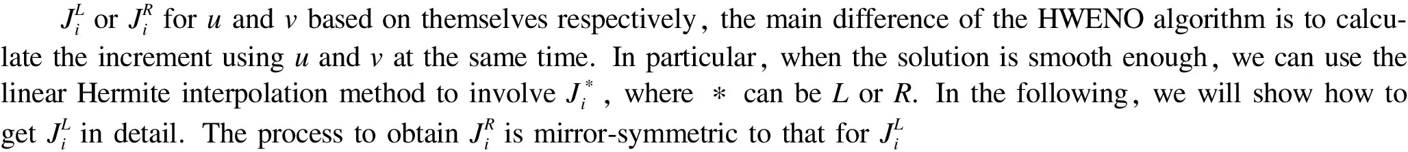
In this paper, we consider to design a suitable hybrid Hermite weighted essentially non-oscillatory (HWENO) for the integral formulation. The main difference of HWENO schemes from WENO schemes is that both the function and its first-order derivative values are evolved in time and used in the integration, not like the WENO schemes in which only the function values are evolved and used in the integration. This allows the HWENO schemes to obtain the same order of accuracy as the WENO schemes with narrower stencils. Hence, less ghost points are needed near the boundaries. Note that the cost of the computation of smoothness indicators and nonlinear weights in HWENO methodology is very high. Hence, we propose the hybrid HWENO scheme in this paper, which can use the optimal linear weights and avoid the computation of the nonlinear weights in the smooth region. Therefore, the hybrid WENO scheme keeps the robustness of the simple WENO scheme, while it is very easy to implement in practice and has higher efficiency.

The rest of the paper is organized as follows. In Section 2, we give the review of the MOLTapproach for one-dimensional linear transport equations. Details of the hybrid HWENO method are given in Section 3. In Section 4, the method is extended to two-dimensional transport equations via dimensional splitting. Several benchmark tests are presented in Section 5 to verify the performance of the proposed scheme, including rigid body rotation, as well as Landau damping, two-stream instabilities, and bump-on-tail for VP simulations. We conclude the paper in Section 6.

2 MOLT framework

In this section, we give a short review of the MOLTframework for the following one-dimensional advection equation,

(2)

wherecis constant denoting the wave propagation speed. The boundary condition is assumed to be periodic, or Dirichlet boundary condition,

(3)

In the MOLTframework, the time variable is discretized at first while leaving the spatial variable continuous. We take the first order backward Euler (BE) method as an example, and obtain

(4)

i.e.,

(5)

un+1(x)=

(6)

where

(7a)

(7b)

An+1andBn+1are constants and should be determined by the boundary conditions. The superscriptL(orR) indicates that the characteristics traverse from the left to the right (or from the right to the left).

To obtain the second order accuracy in time, we can use the Crank-Nicolson (CN) time discretization on 920 and obtain the semi-discrete scheme

(8)

Based on the similar idea, solution of the BVP (8) can be given analytically,

(9)

For both semi-discrete schemes (6) and (9), we need to further discretize the spatial variable. Suppose the domain [a,b] is discretized byM+1 uniformly distributed grid points

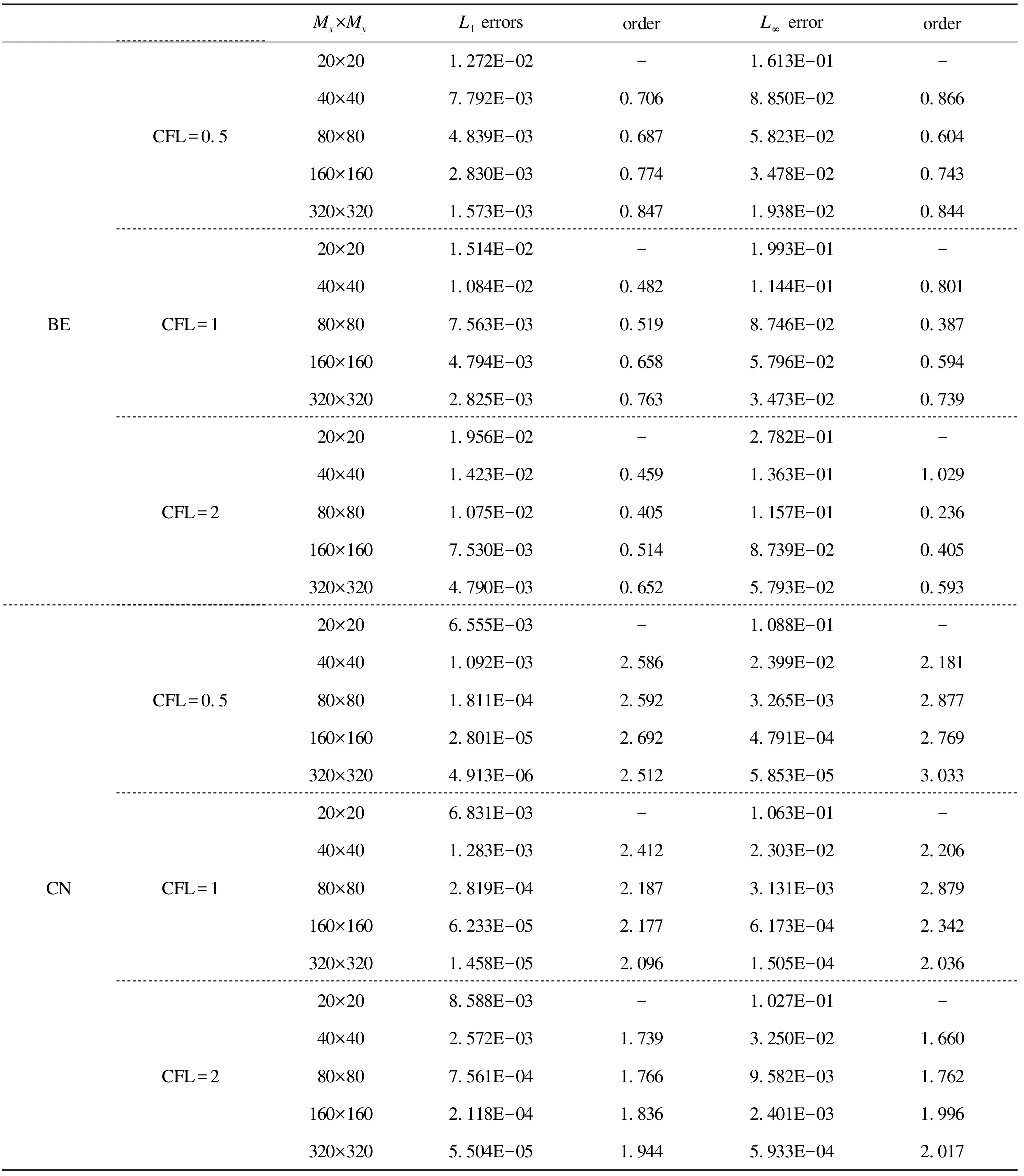
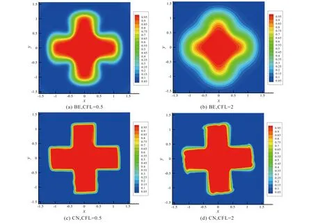
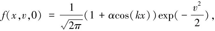
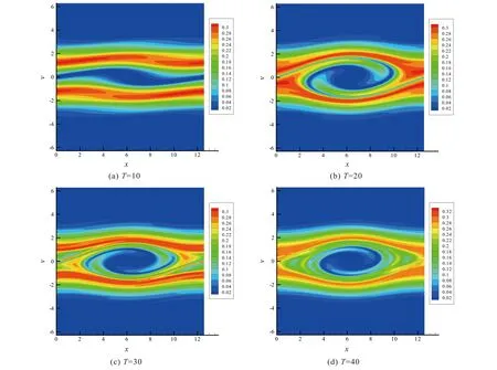
a=x0

(10a)

(10b)

where

(11)

An+1=g1(tn+1), orBn+1=g2(tn+1)

(12)

when coupling with the BE scheme (6), or

(13)

when coupling with the CN scheme (9). For the periodic boundary condition, the coefficients can be determined by using the mass conservation property of the solutions, which leads to

(14)

or

(15)

3 HWENO methodology

The HWENO has been widely studied to solve the hyperbolic conservation laws in MOL framework, including the finite difference method[28-30], the finite volume method and the nonlinear limiter for the discontinuous Galerkin (DG) method[31-34]. Here, we will use the idea to approximate the integration.

In the Hermite framework, both the function and its spatial derivative are needed to be evolved in time. Denote the spatical derivative of functionu(x,t) asv(x,t). Then from (2) and its spatial derivative, we have the governing equation:

Ut+cUx=0

(16)

where

The boundary conditions can be obtained corre-spondingly, for instance, Dirichlet boundary condition

(17)

Note that each component of system (16) satisfies the 1D advection equation (2). Hence, we can apply the MOLTframework introduced in Section 2 directly onuandvrespectively. For instance, whenc>0 and coupling the BE scheme, we have

(18a)

(18b)

Here, taking the stencilS={ui-1,ui,vi-1,vi} as an example, there is a unique Hermite interpolation polynomialp(x) of degree at most 3, such that

p(xj)=uj,p′(xj)=vj,j=i-1,i.

Then, we can obtain that the approximations

(19)

(20)

withγ=αΔx. The schemes (19) and (20) will give us third order accuracy in space. It is worth noting that we can perform the integration by parts (IBP) to the polynomialp(x), and obtain that

which means

(21)

(22)

The main procedures of the hybrid HWENO scheme are given as follows. On each cell, we will identify the troubled cell. However, different troubled-cell indicators may have different effects for the hybrid HWENO scheme. Here, we follow the idea in Ref.[30,35] that looking at the locations of all extreme points of the big interpolation polynomial. Then calculate the integrations by HWENO approximation in troubled cell and linear approximation in other regions. A series of unequal-sized hierarchical stencils are used in designing high order HWENO schemes. This kind of unequal-sized hierarchical stencils WENO scheme is proposed in Ref.[36] for solving hyperbolic conservation laws with the good properties such as the linear weights can also be any positive numbers if their sum equals one.

Algorithm 3.1The hybrid HWENO method for the 1D system (16).

If all of the extreme points ofp(x) andp′(x) are outside the intervalIi=[xi-1,xi], which means the polynomials are monotone in this cell, then we will use linear schemes (19) and (21).

Step 2.1On each candidate stencilSr, construct (Hermite) interpolation polynomials with degree at most 2r-1, denoted bypr(x). The integration can be approximated by

(23)

In particular,

Step 2.2Obtain equivalent expressions for these (Hermite) interpolation polynomials of different degrees, denoted byqr(x).

(24)

withθ2>0,θ1≥0 andθ1+θ2=1. Moreover, we can define a linear weightdr=θr,r=1, 2, such that

p2(x)=d1q1(x)+d2q2(x).

q2(x)=1.01p2(x)-0.01q1(x).

Moreover, we can obtain the corresponding integral

In particular,

Step 2.3Compute the nonlinear weights based on the linear weights and the smoothness indicatorsβr, which are given as

The explicit formulations ofβrare given as following,

β1=(ui-1-ui)2,

And we can obtain the nonlinear weights as

(25)

where

(26)

Step 2.4Finally, the integral can be obtained as

(27)

and

withγ=αΔx.

(28)

Step 3.3Compute the nonlinear weights based on the linear weights and the smoothness indicators.

(29)

where

and the linear weights are given as

(30)

Note thatp2(x) is the interpolation polynomial obtained in Step 2.

Step 3.4The new approximation is given by

Remark 3.2The exact solutionuof (16) satisfies the boundary-preserving principle, meaning that if the initial conditionm≤u(x,0)≤M, then the exact solutionm≤u(x,t)≤Mfor any timet>0. To maintain the numerical schemes also satisfy such a property on the discrete level, we will employ the boundary-preserving limiter introduced in Ref.[12]. It can work for both periodic and Dirichlet boundary conditions. Details would not be given here.

4 Two-dimensional implementation

In this section, we extend the algorithm to two-dimensional problems in the following form:

(31)

For the Hermite method, we give not only the solutionubut also its derivatives inx- and iny-directions. We have the following equations foruxanduy,

(32)

In this paper, the system (31) and (32)are solved based on the Strang splitting method[8], which gives us the second order accurate in time. Firstly, we decouple the 2D system (31) and (32) into a sequence of independent 1D systems

(33)

and

(34)

SupposeQ1andQ2be the approximate solvers for each system, that isUn+1=Q1(Δt)Unis an approximation of (33), andUn+1=Q2(Δt)Unis an approximation of (34), withU=(u,ux,uy)T. Then, second order semi-discrete scheme for one step evolution fromUntoUn+1can be achieved in by employingQ1andQ2consecutively,

(35)

Note that, the first two equations in system (33) and (34) can be solved by the 1D MOLT-HWENO method given in Section 3. However, the third equations need different treatment. Here, Below, we focus our discussion on the solverQ1for (33). The solverQ2and would be similar.

Let (xi,yj) be the node of a 2D orthogonal grid with uniform mesh size in each direction

ax=x0

ay=y0

Algorithm 4.1The solverQ1(Δt) for the system (33).

Step 2Apply the same time discretization on (FDx). For instance, when using the BE method, we have that

Or we can obtain the following semi-discrete scheme when employing the CN time discretization,

where * can benorn+1.

Note that the 1D1V VP system can be split into two systems as well

(36a)

and

(36b)

Similarly, the VP system can be approximated by the Strang splitting method. And the electrostatic fieldE(x,t) is obtained by solving Poisson’s equation when it is needed.

5 Numerical results

In this section, we present the numerical results with the schemes described in the previous sections. Both backward Euler (BE) scheme and Crank-Nicolson (CN) scheme are used in time discretization, coupling with the 4-point hybrid HWENO integration. For 2D problems the time steps are chosen as

Δt=CFL/max(|cx|/Δx,|cy|/Δy)

(37)

5.1 Basic 2D test

Here, we consider the rigid body rotation problem.

(38)

with two different initial conditions:

① continuous initial condition:

(39)

where

u(x,y,0)=

We simulate both problems with periodic boundary condition and zero Dirichlet boundary condition.

In Tables 1 and 2, we summarize the convergence study of the continuous problem at the final timeT=2π, where the exact solution is as the same as the initial condition. The norm of the error is computed according to

Table 1. Under periodic boundary condition, errors and orders of accuracy for solving (38) with continuous initial condition (39) at T=2π.

Table 2. Under Dirichlet boundary condition, errors and orders of accuracy for solving (38) with continuous initial condition at T=2π.

whereue(xi,yj,t) denotes the exact solution. We test both the BE scheme and the CN scheme with CFL=0.5, 1, 2. We can see that all schemes are stable and converge to the designed order of accuracy. Moreover, when using CN scheme with CFL=2, numerical results show higher order than 2. This because spatial errors play a leading role in errors due to the small time step, and the 4-point HWENO scheme is third order accuracy.

For the discontinuous problems, we test our scheme with CFL=0.5 and 2. The HWENO methodology removes unphysical oscillations as expected (Figures 1 and 2). And the CN schemes give sharper interface than the BE schemes.

Figure 1. Under periodic boundary condition, numerical solutions for solving (38) with discontinuous initial condition at T=2π. 160×160 grid points.

Figure 2. Under Dirichlet boundary condition, numerical solutions for solving (38) with discontinuous initial condition at T=2π. 160×160 grid points.

5.2 The VP systems

Here, we will consider the Vlasov-Poisson equation (1) with the following initial condition:

① Strong Landau damping:

x∈[0,L],v∈[-Vc,Vc],

whereα=0.5,k=0.5,L=4πandVc=2π.

② Two-stream instability I:

x∈[0,L],v∈[-Vc,Vc],

whereα=0.01,k=0.5,L=4πandVc=2π.

③ Two-stream instability II:

x∈[0,L],v∈[-Vc,Vc],

whereα=0.05,k=0.5,L=4πandVc=2π.

④ Bump-on-tail instability:

0.2exp(-4(v-4.5)2)),

x∈[-L,L],v∈[-Vc,Vc],

In our numerical tests, the periodic boundary condition is imposed inx-direction and the zero boundary condition is imposed inv-direction. A fast Fourier transform (FFT) is used to solve the 1D Poisson equation. We only test the VP systems with the CN scheme and CFL=1. Numerical results are plotted in Figures 3-6. It is observed that solution will develop filamentation solution structures after a long time evolution, and the scheme is able to effectively capture those structures without producing spurious oscillations.

Figure 3. Strong Landau damping. 128×256 grid points.

Figure 5. Two-stream instability II. 128×256 grid points.

Figure 6. Bump-on-tail instability. 128×256 grid points.

6 Conclusions

In this paper, we proposed a new type hybrid Hermite weighted essentially non-oscillatory (HWENO) schemes coupled with the implicit method of lines transpose (MOLT) framework for the Vlasov-Poisson (VP) system for plasma simulations. The main idea of the hybrid HWENO scheme is that if all extreme points of the big interpolation polynomial and its derivative are located outside of the big stencil, then we will use linear approximation straightforwardly to increase the efficiency of the scheme, otherwise use the HWENO procedure to avoid the oscillations nearby discontinuities. The algorithm was extended to multi-dimensional problems and the VP system via dimensional splitting. Comparing them with the WENO-based MOLTschemes[23], the new HWENO-based MOLTschemes are more efficient and compact, hence, less ghost points are needed near the boundary. In this paper, we consider the first order backward Euler scheme and the second order Crank-Nicolson scheme, coupling with a 4-points HWENO integration, which are unconditionally stable. A collection of numerical tests demonstrated good performance of the proposed scheme. Higher order numerical scheme will be considered in the future.

Acknowledgments

The work is supported by National Natural Science Foundation of China(Nos. 11901555, 11871448).

Conflictofinterest

The authors declare no conflict of interest.

Authorinformation

WangKaipengis currently a PhD candidate under the tutelage of Prof. Jiang Yan and Prof. Zhang Mengping at University of Science and Technology of China. His research interests focus on numerical solution of partial differential equation and big data science.

JiangYan(corresponding author) is a Research Professor at School of Mathematical Sciences, University of Science and Technology of China (USTC). She received her PhD degree in computational mathematics in 2015 from USTC. From 2015 to 2018, she worked as a Postdoctoral Fellow at Michigan State University. In 2018, she joined USTC. Her research area is numerical analysis and scientific computing.