Solid solution strengthening in multicomponent fcc and bcc alloys:Analytical approach

M.Lugovy,V.Slyunyayev,M.Brodnikovskyy

Institute for Problems of Materials Science,Kiev,Ukraine

Keywords:Multicomponent alloy Solid solution strengthening model Atomic size misfit Elastic modulus misfit

ABSTRACT Based on virtual solvent concept,novel methods are developed to determine interatomic distance,atomic size misfit,and elastic modulus misfit in multicomponent alloys with components having the crystal structure differing from that of the alloy.The combination of the different methods results in a number of models to calculate solid solution strengthening.These models are assessed with view point of the best fit to experimental data.The models giving the most reliable strengthening prediction can be used for an evolutionary design of strong and stable multicomponent alloys.

1.Introduction

Multiprincipal element alloys(MPEAs)are multicomponent metal systems with comparable concentrations of the alloy components[1-3].The properties of such alloys are strongly dependent on the number of components.The high strength of such materials is often combined with good plastic characteristics[4-8].The combination of good mechanical properties,microstructural stability as well as high oxidation and corrosion resistance makes them very promising for practical applications[9-11].

The majority of MPEAs are multiphase materials.However,there are also single-phase solid solution alloys [5,7,8,12-29].The formation of such a structure can be explained by an increase in the configuration entropy,retarded diffusion in the highly distorted lattice,and the so-called cocktail effect which stabilizes the solid solution[1,3,4].

The MPEAs strength is determined by solid solution,grain size,dispersion,and order strengthenings[16,30,31].Only the solid-solution and grain-size strengthenings are essential for single-phase alloys.As regards the order strengthening,it can be neglected in the majority of MPEAs [32,33].The solid-solution strengthening (SSS) is considered to be a major contribution to the yield strength of the alloys.For example,a relative contribution of the SSS is about 50% of the yield strength in AlxCoCrCuFeNi alloys [31].

The solid-solution strengthening is based on the interaction of dislocations with solute atoms.This interaction is primarily determined by the atomic size misfit as well as the elastic modulus one [34].Models of solid-solution strengthening for a binary alloy were worked out in Refs.[35,36].The Fleischer model assumes the presence of single noninteracting atoms[35].This model is applicable to dilute solid solutions.The Labuschmodel applies to the concentrated ones[36].The model considers that solute atoms can be nonuniformly distributed giving rise to the groups of the above relatively closely spaced atoms.The Fleischer and Labusch models are mainly distinct in employing different methods of statistical averaging of the dislocation interaction with solute atoms.Solid solutionstrengthening due to severalnoninteractingsolutes is shown to be equivalent to the strengthening from one effective solute[37].

The methodology[37]was used in Ref.[16,20,38-43]to describe the SSS in MPEAs.Such alloys do not contain any physically distinguished solvent.All alloy components are equivalent.Therefore,the interatomic distance has a deviation from the average lattice parameter,induced by an individual constitutive element,instead of changing the lattice parameter of the solvent due to the solute.Other models of the SSS in MPEAs were also elaborated in Refs.[44,45].The model [44] is only applicable to fcc alloys.The model [45] relies upon the strengthening parameters obtained from experimental hardness data for the specific pairs of components.Therefore,the models[44,45]are not examined in this paper.

The major problem of modelling the SSS in MPEAs is a calculation procedure for the atomic size and shear modulus misfits.There are several approaches to calculate the shear modulus and atomic size misfits[8,12,16,39,41,43].Sometimes the atomic radii or lattice parameters of pure elements are used to estimate the atomic size misfit [8,12,16,41].The atomic radius or lattice parameter should be corrected with the pure element lattice differing from that of MPEAs.Known correction methods can be considered only as the first approximation[12,41].The distance between the nearest atoms is more appropriate entity to calculate the atomic size misfit [39,40].Generally,the distance between the same nearest atoms in the alloy differs from that of the lattice in a corresponding pure element.The interatomic distance matrix describing the average distance between different atoms in the alloy was defined in Ref.[46].The methods based on the interatomic distance matrix other than the published ones may also be proposed to calculate the atomic size misfit.It should be noted that the combination of different calculation procedures for atomic size and shear modulus misfits gives rise to a wide variety of SSS models.

Note that fcc and bcc lattice alloys exhibit different SSS patterns for the same atomic size and shear modulus misfits.It can be associated with a different number of slip systems in both crystal structures [39].All models contain fitting constants,which relate the misfits and shear modulus of the alloy to its SSS.Separate examination of fcc and bcc alloys is best suited for determining the fitting constant of the model.

Reliable SSS prediction is a key factor for an evolutionary design of strong and stable MPEAs with multiobjective optimisation based on physical models,statistics,and thermodynamics.One of the algorithms of such a design is presented in Ref.[47].Therefore,it is of first importance to evaluate SSS models for establishing the most accurate ones.The goal of this study is to develop the methods to determine interatomic distance,atomic size misfit,and elastic modulus misfit in multicomponent alloys with components having the crystal structure differing from that of the alloy,to assess corresponding SSS models with the view point of the best fit to experimental data.

2.Solid solution strengthening models

The solid-solution strengthening of a multicomponent alloy can be generally described as[16,39].

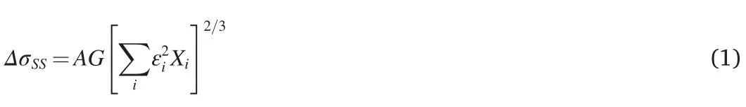
where A is the fitting constant,which can be found from the comparison of calculated and experimental SSS data,Gis the shear modulus of the multicomponent alloy,Xiis the atomic fraction of the component i in the alloy,is the shear modulus of the pure component i,εi,α is the constant dependent on the type of dislocations responsible for plastic deformation(it is usually assumed that 3 ＜α ＜16 for the screw dislocations and α ＞16 for the edge dislocations),is the elastic modulus misfit,δiis the atomic size misfit,slatis the average distance between the nearest atoms in the multicomponent alloy.Eq.(1) is based on the concept [33] that treats the multicomponent alloy as a virtual homogeneous material consisting of identical“average”atoms with the average distance between the nearest atoms in equilibrium slat(virtual solvent) and all components of the alloy are seen as the effective virtual solutes.It is the modification of the concept [37].There are at least two procedures to calculate ηiand numerous ones to calculate δi.Thus,there are several ηiand δicombinations to calculate εi.Each combination can be regarded as a model to describe the SSS in the multicomponent alloy.

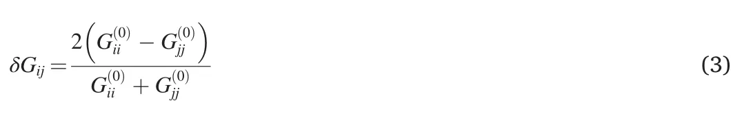
The first model to calculate ηi(Case G1)[8,12].

where p is the coefficient (p13/12 for the fcc,andp9/ 8 for bcc alloys),

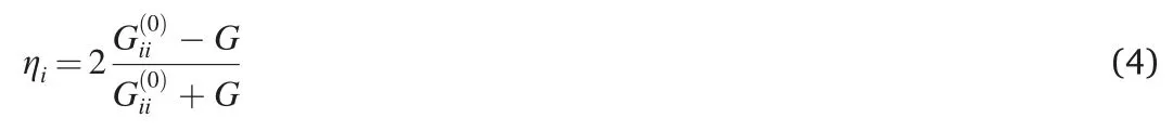
The second model to calculate ηi(Case G2)[39].

The first model to calculate δi(Case R1)[12].

where

Riiis the distance between the nearest atoms in equilibrium in the lattice of the pure component i[16].It should be noted that Eq.(6)at Riiis valid only for the same type of the lattice in the alloy and its components.Otherwise,should be corrected to correspond to the event of the component i having the same lattice as the alloy one.Such a correction can be thought of only as the first approximation.Therefore,Riiis rather inadequate for calculations.Another model to calculate Riiis Riisii/2,where siiis the average distance between the nearest atoms of the component i in the lattice of the multicomponent alloy.Riisii/2 is valid for different types of the lattice in the alloy and its components.The siievaluation as well as the average distance between the nearest atoms of the components i and j in the lattice of the multicomponent alloy sijis presented in the Section3.

Another model of calculating δi(Case R2)[39].

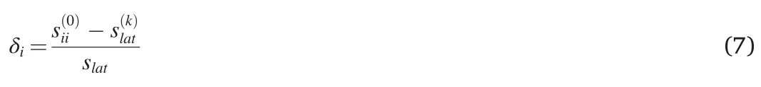
If the element i is removed and the atomic fractions of other components are replaced,respectively.The distances sijin form of the matrix S（sij）.The original composition of the alloy is determined by the row vector X（X1，...，Xi，...，Xj，...，XN）.The superscript T designates the transpose operation transforming the row vector into the column one.The slatvalue varies from slatfor the pure component i(Xi1)to slatfor the special multicomponent alloy without the component i (Xi0).

The next model to calculate δi(Case R3)

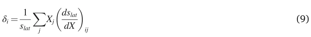
where

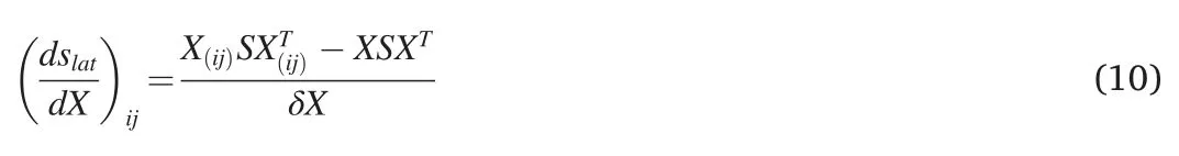
is the slatvariation by removing one atom of the type j and replacing it with an atom of the type i,δX is a very small change of the atomic fraction(corresponding to one atom in the ideal case but simply a very small value in practical calculations),a modified composition of the alloy is determined by the row vector X（ij）（X1，...，Xi+δX，...，Xj-δX，...，XN）.The parameterdetermines slatcorresponding to the modified composition X（ij）.

The parameter δican be also calculated as(Case R4)

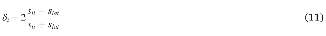
Here δiis calculated similar to the elastic modulus misfit ηi(Case G2-see(4)).

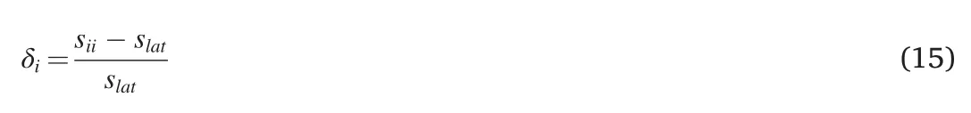
The solid solution strengthening of a multicomponent alloy can be described as in Ref.[41].

where

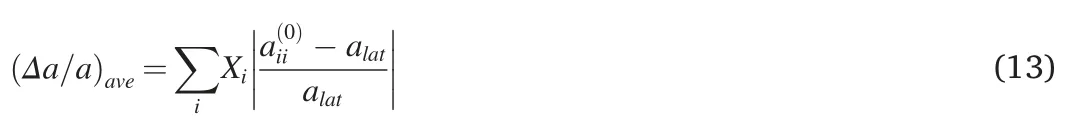
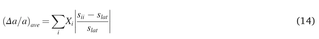
Eq.(14) is valid for the alloy and component lattices of different types.Note that in this case we should consider(Case R5)

The solid solution strengthening of a multicomponent alloy can also be described in the matrix form [43].The contribution of Bijdue to the interaction of the atoms of types i and j can be taken into account proportionally to the frequency of possible interactions i-j’ which equals XiXj.It is also assumed that the interactions i-i and j-j of the frequencies XiXiand XjXjrespectively,do not have any effect on the SSS,i.e.,BiiBjj0.Then

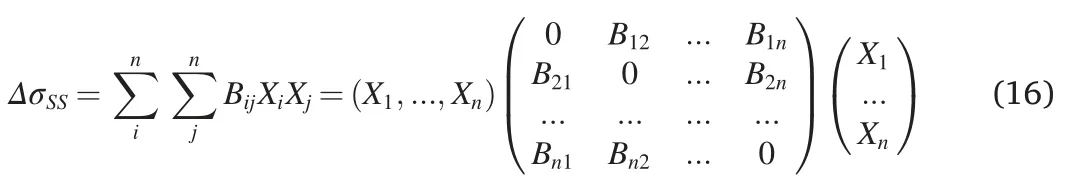
where

and

Note that in this case we can derive from Ref.[43] (Case R6)

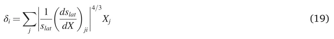
The combinations of G1,G2,R1,R2,R3,R4 to determineηiand δigive eight versions of the εicalculation:G1R1,G1R2,G1R3,G1R4,G2R1,G2R2,G2R3,G2R4.Correspondingly,there are eight models in the framework of Eq.(1) to calculate solid solution strengthening.The two models which use Cases R5 and R6 to calculate atomic size misfit do also exist.Note that the last two models are not based on Eq.(1)and the shear modulus misfit is neglected in them.All the examined models in terms of ηiand δiare summarized in Table 1.The flowchart of SSS calculation is presented in Fig.1.

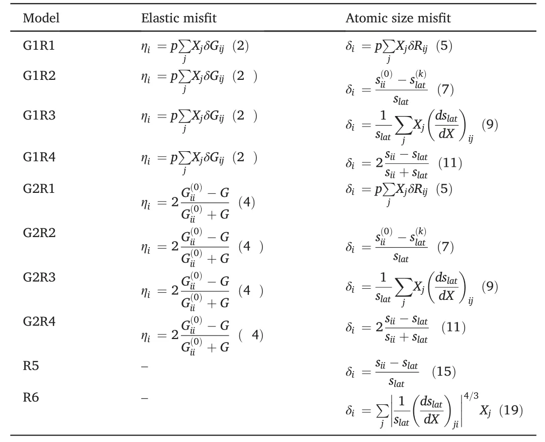
Table 1 Examined models.

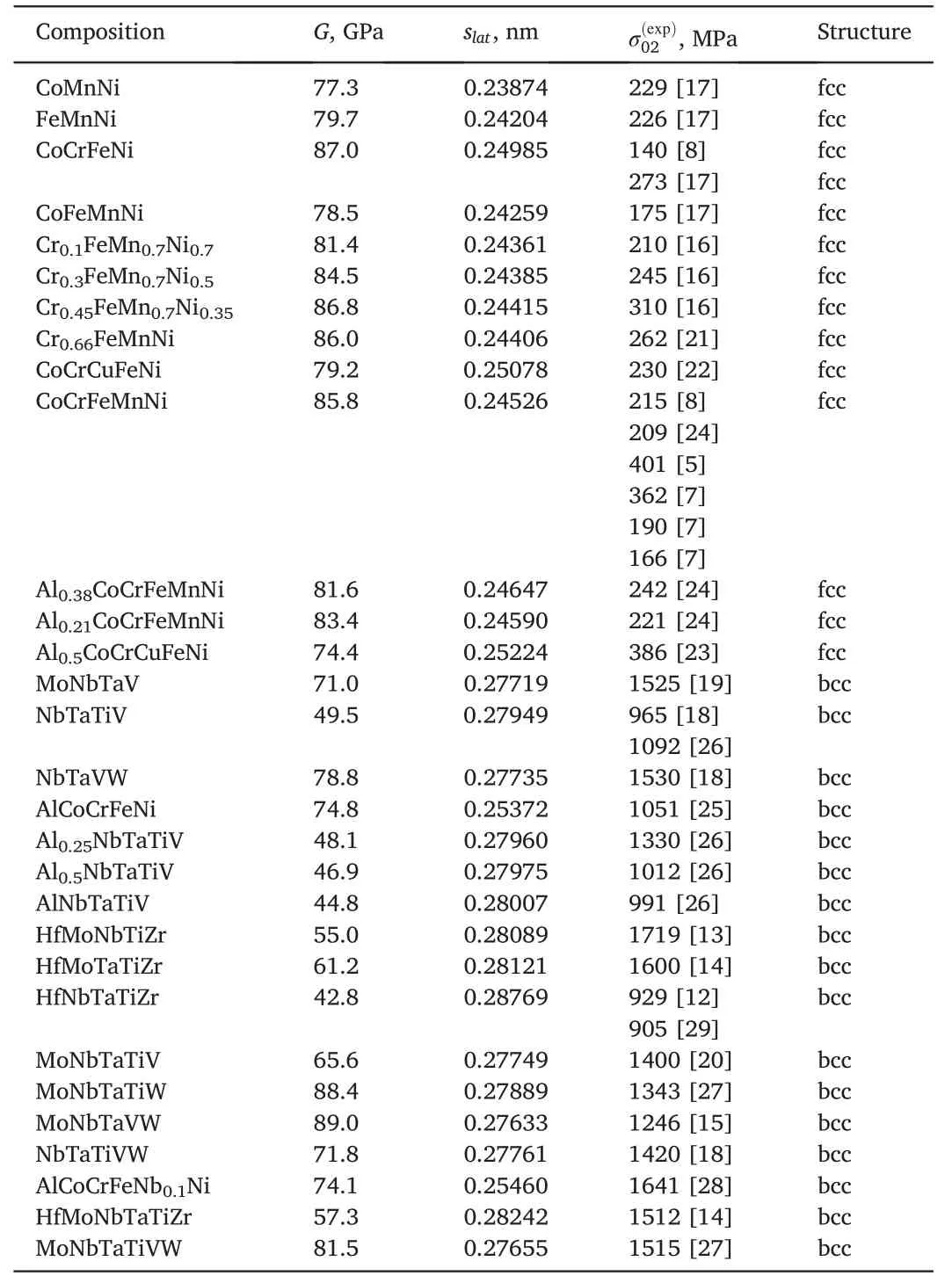
Table 2 Multicomponent alloys for model verification.

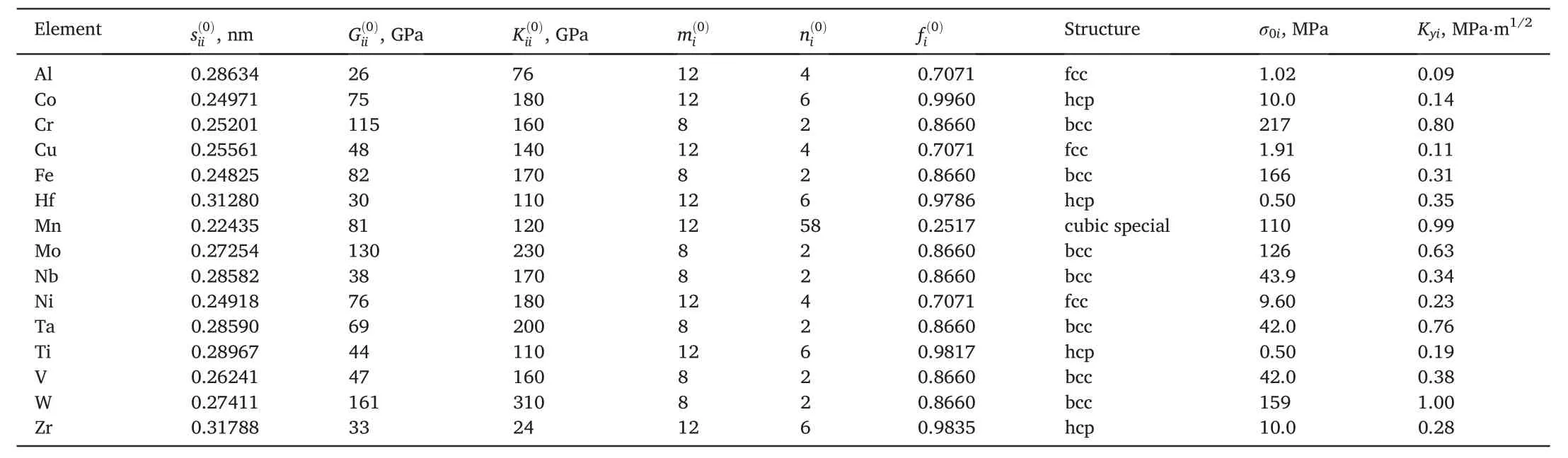
Table 3 Component characteristics.The friction stress of dislocation motionσ0 and the grain-size strengthening coefficient Ky for the alloy may be estimated with Vegard’s law[31].

3.Interatomic distance

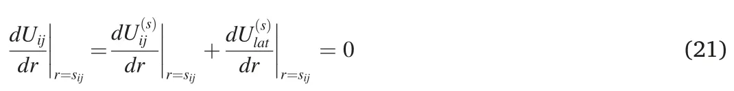
The potential energy of an atom in the lattice of a multicomponent alloy is provided by the interactions of neighboring atoms,mainly the nearest ones,and is dependent on the distance r between the atoms.Its minimum determines the average distance between the nearest atoms at equilibrium.The average distance sijbetween the atoms of the components i and j in the lattice of the multicomponent alloy is defined by the potential energy of corresponding i -j interactions:

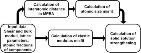
Fig.1.The flowchart of SSS calculation.

In the binary subsystem,we have

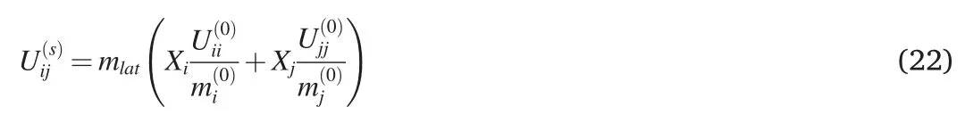
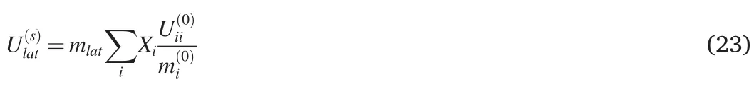
where mlatis the coordination number in the lattice of the alloy,is the interatomic potential in the lattice of the pure component i,is the coordination number in the lattice of the pure component i(mlat8 for the bcc lattice and mlat12 for the fcc lattice).Note thatis approximately the potential energy per one interatomic interaction in the lattice of the pure component i.is the average sum of the contributions of the i -j interactions.In this case the atoms of other components are regarded as“vacancies”,viz.empty sites.Based on virtual solvent concept,the average potential energy of an atom in the lattice of the multicomponent alloy without considering the i-j interactions is

The interatomic potential in the lattice of the pure component i can be approximated by the quadratic function near the equilibrium atomposition:

where p1i,p2i,and U0，iiare the constants.The bulk modulus of the pure component i can be expressed as[40]:

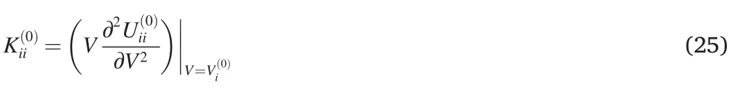
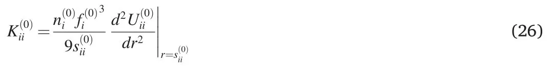
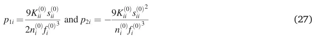
Similar to Eq.(24),we can also expressandas

where as Eq.(27)

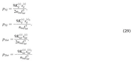
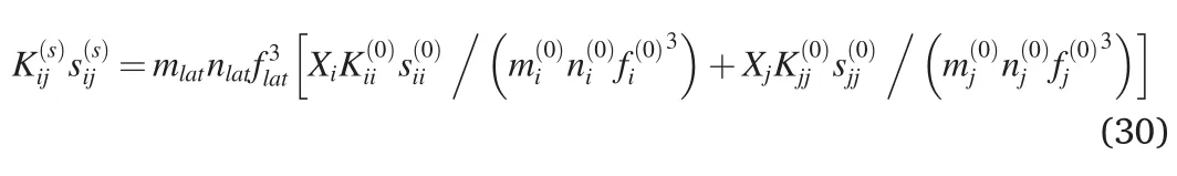
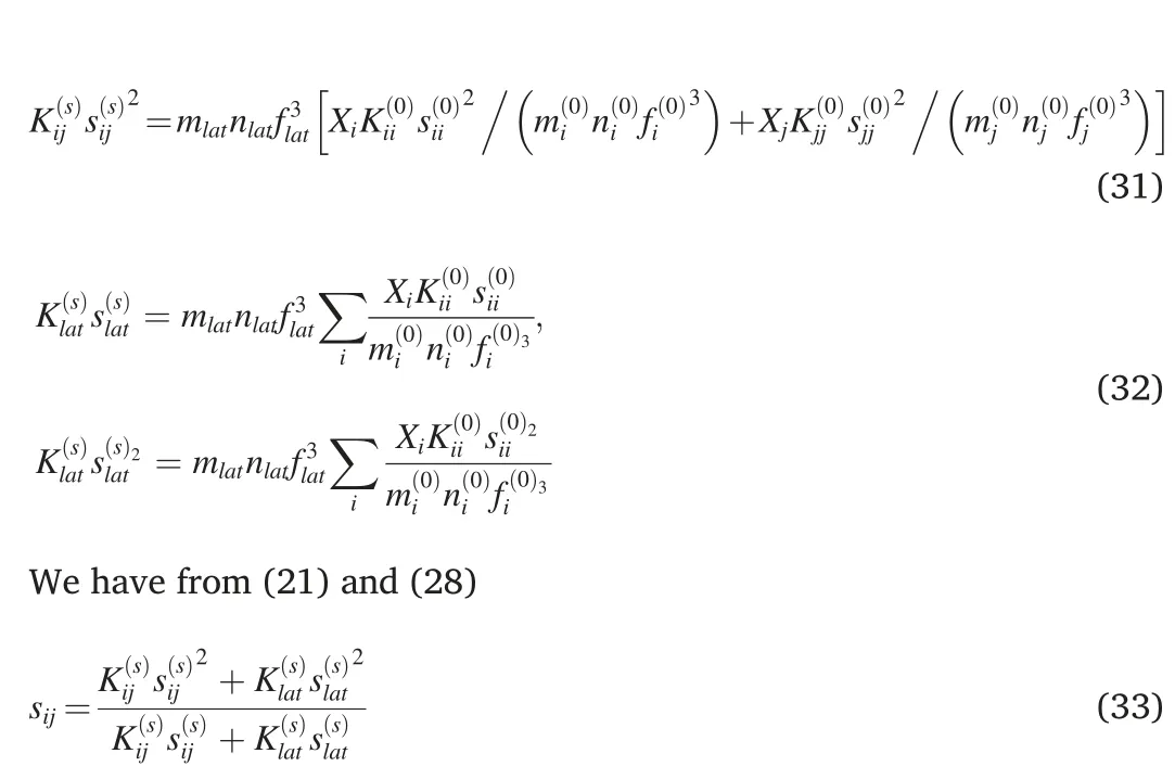
Eq.(33)is similar to Eq.(27)in Ref.[40].But in view of(30)-(32),Eq.(33) is more general because it uses the average distance between the nearest atoms instead of lattice parameter in Eq.(27)of[40].Eq.(33)is valid for different lattice types in the alloy and its components.Eq.(27)in Ref.[40] is valid only for the same lattice type in the alloy and its components.Eq.(33) yields sii,if ji.Note that sii/s（0）ii.The average distance between the nearest atoms of the component i in the lattice of the multicomponent alloy siiis shifted to such a distance in the multicomponent alloy slatdue to the influence of other atoms[40].The lattice parameters of alloys CoNi,FeNi,Ni4Pd,CoCrNi,CoFeNi,CoMnNi,FeMnNi,CrFe2Ni2,CoCrFeNi,CoCrMnNi,CoFeMnNi,CoCrFeNiPd,(CoCrFeNi)0.99Pd0.01,(CoCrFeNi)0.97Pd0.03,(CoCrFeNi)0.95Pd0.05calculated using the above approach is found to be in good accord with experimental data[48-50].

4.Model assessment

The 13 fcc and 17 bcc structure of multicomponent alloys were chosen to verify the above models of SSS with defining the best one(Table 2).The choice is governed by the following:(i)the alloy should be a single-phase solid solution and(ii) the yield point obtained in tension and/or compression tests of this alloy should be available.The characteristics of the alloy components are given in Table 3.Note that σ0iand Kyiare the friction stress of dislocation motion and the grain size strengthening coefficient for the element i,respectively.Theσ0ivalues for Co,Cu,Fe,Nb,and Ni were evaluated from the critical resolved shear stress of these elements in Refs.[31,51-54],respectively.For other elements σ0iwas estimated with[17,55].

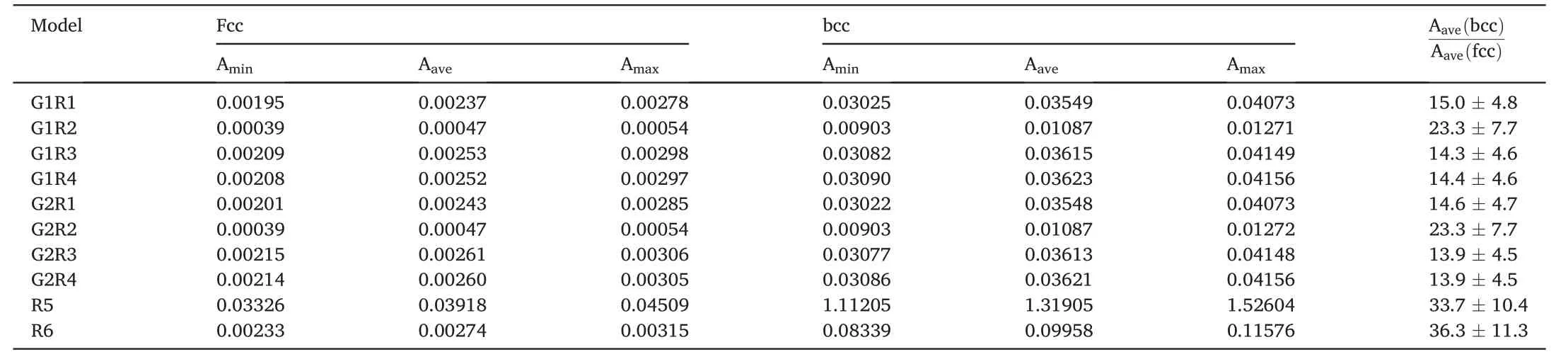
Table 4 Fitting constant estimates for examined models.

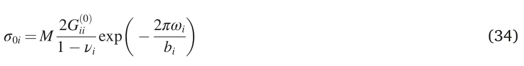
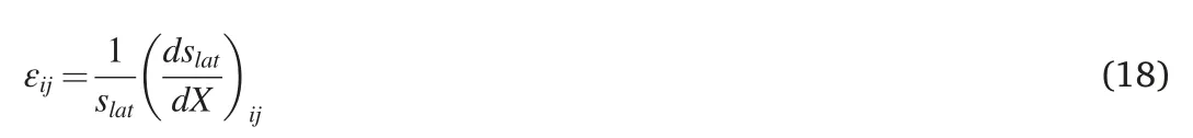
where M is the Taylor factor(assumed to be 3.06 and 2.75 for the fcc and bcc metals,respectively[55]),νiis Poisson’s ratio,biis the Burgers vector,ωiis the temperature-sensitive dislocation width of the component i.Eq.(34) is valid for different temperatures if corresponding ωiis used.Note that ωi/bidepends on a crystal lattice type(ωi/biis evaluated to be about 1.9 for the fcc and hcp metals and about 1.4 for the bcc metals at room temperature based on measured σ0i[31,51-54]).The Kyivalues are presented in Ref.[56].

It was found that the friction stress for some alloys estimated with Vegard’s law was in good accord with σ0evaluated by other methods[7,17].The alloy may be treated as a virtual solvent,i.e.,the ideal material with an“average”lattice [33].The friction stress is strongly dependent on the alloy composition and temperature.

The lower and upper boundaries of grain-size strengthening in the alloys can be calculated using the Hall-Petch equation[31].

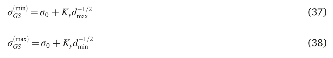
where dminand dmaxare the minimum and maximum estimates of actual average grain size in the alloy.The dminand dmaxvalues were evaluated from the microstructure images [5,7,8,12-29].In the alloys of the dendrite structure,the secondary dendrite arm spacing was used instead of the grain size.Scattering of grain size data leads to certain inaccuracy in determining the grain size strengthening.Then experimental minimum,maximum,and average estimates of SSS in the alloy may be expressed as

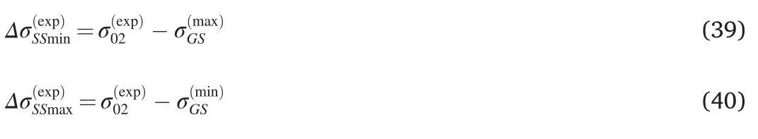
Fig.2.Computed solid solution strengthening versus its experimental values(defined from the yield strength):A,C,E-fcc alloys;B,D,F-bcc alloys;A,B-G1R1 model;C,D-G1R3 model;E,F-G1R4 model.Horizontal and vertical error bars show uncertainty of determining the experimental and computed SSSs,respectively.

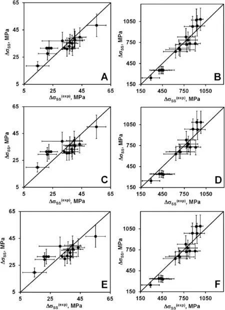
Fig.3.Computed solid solution strengthening versus its experimental values(defined from the yield strength):A,C,E-fcc alloys;B,D,F-bcc alloys;A,B-G2R1 model;C,D-G2R3 model;E,F-G2R4 model.Horizontal and vertical error bars show uncertainty of determining the experimental and computed SSSs,respectively.

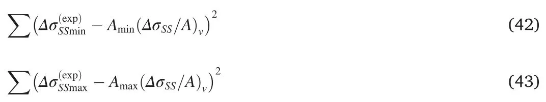
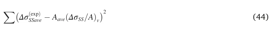
Fig.4.Computed solid solution strengthening versus its experimental values(defined from the yield strength):A,C-fcc alloys;B,D-bcc alloys;A,B-G1R2 model;C,D -G2R2 model.Horizontal and vertical error bars show uncertainty of determining the experimental and computed SSSs,respectively.

In the fcc alloys,fitting constants values lie in the range of 0.00195-0.00306 for G1R1,G2R1,G1R3,G2R3,G1R4,G2R4 models and in the range of 0.00039-0.00054 for G1R2,G2R2 models.These values for R5 and R6 models are within 0.03326-0.04509 and 0.00233-0.00315,respectively.In the bcc alloys,the constants are within 0.03022-0.04156 for G1R1,G2R1,G1R3,G2R3,G1R4,G2R4 models and in the range of 0.00903-0.01272 for G1R2,G2R2 models.These values for R5 and R6 models lie in the ranges of 1.11205-1.52604 and 0.08339-0.11576,respectively.Note that the fitting constant of a G1R1 model for the bcc alloys is close enough to that of the refractory bcc alloys in Ref.[55].The ratio of the fitting constants for bcc and fcc alloys is about 14.6±5.2 for G1R1,G2R1,G1R3,G2R3,G1R4,G2R4 models,23.3 ±7.7 for G1R2,G2R2 models and 35.5± 12.1 for R5,R6 models.Hence the models can be divided into the three groups.Note that the fitting constants for the bcc alloys are substantially larger as compared to those of the fcc alloys.Therefore,the bcc alloys exhibit a higher SSS for the same atomic size and shear modulus misfits than the fcc alloys.It can be explained by a different number of active slip systems in the two crystal structures[39].

Fig.2 shows the solid solution strengthening computed with G1R1(A,B),G1R3 (C,D),and G1R4 (E,F) models versus its experimental values based on the yield strength of the fcc(A,C,E)and bcc(B,D,F)alloys.Note that the SSS values for the fcc alloys are much smaller than those of the bcc alloys.The above small values for the fcc alloys was also observed in Ref.[57].Moreover,the solid solution strengthening obtained in this study is low as compared to that computed in other investigations for the fcc alloys[33,43].It can be explained by a strong underestimation of the friction stress of multicomponent fcc alloys or the friction stress inclusion into the SSS value,neglecting the athermal component in those studies.In particular,such an underestimation can be associated with neglect of a narrowing dislocation width in a multicomponent fcc alloy in comparison with pure fcc metals[7,17].Subject to some data uncertainty,computed and experimental strengthenings demonstrate good agreement.

Fig.3 presents the solid solution strengthening computed with G2R1(A,B),G2R3 (C,D),and G2R4 (E,F) models versus its experimental values defined from the yield strength of the fcc(A,C,E)and bcc(B,D,F)alloys.As is seen,G2R1,G2R3,and G2R4 models give the results that are very similar to those of the G1R1,G1R3,and G1R4 models.The above two groups of models differ only in the computation method for the elastic modulus misfit (Cases G1 and G2).Similarity of the results indicates that those methods to calculate the misfit differ insignificantly.

Fig.4 A,B and 3C,D present respectively the solid solution strengthening computed with G1R2 and G2R2 models versus its experimental values.Results for the fcc and bcc alloys are depicted in Figs.4A,C and 3B,D,respectively.As is seen,the agreement between computed and experimental data is poorer than in the case of G1R1,G1R3,G1R4,G2R1,G2R3,G2R4 models,especially for the bcc alloys.The bcc alloys are divided into the three groups (Fig.4).The group with the least strengthening shows a fairly good agreement between the computed and experimental values.The other two groups have approximately the same experimental strengthening values but significantly differing computed ones.

Fig.5 shows the solid solution strengthening computed with R5(A,B)and R6 (C,D) models versus its experimental values defined from the yield strength of the fcc(A,C)and bcc(B,D)alloys.Similar to G1R2 and G2R2 models,the agreement between computed and experimental strengthenings is poor for those two models as compared to G1R1,G1R3,G1R4,G2R1,G2R3,G2R4 models,especially for the bcc alloys.

Fig.5.Computed solid solution strengthening versus its experimental values(defined from the yield strength):A,C-fcc alloys;B,D-bcc alloys;A,B-R5 model;C,D-R6 model.Horizontal and vertical error bars show uncertainty of determining the experimental and computed SSSs,respectively.

The level of correspondence between computed and experimental data can be evaluated with the sums of squared deviations of those values.The sums can be calculated with Eq.(44).Since the sums are dependent on the examined alloys,they should be normalized for comparison.Fig.6 presents normalized sums of squared deviations for the examined models.The sums were normalized corresponding to the R6 model for the fcc and bcc alloys separately which equals unity in Fig.6A and B.In both fcc and bcc alloys,the normalized sums are less than unity for all other models.The smaller this sum is,the better the agreement between the computed and experimental strengthenings will be.In the view of their small difference,the modelwith the best fit isdifficult tobe establisheddue to some uncertainty of the sums.The models for the fcc alloys are therefore divided into the two groups:G1R1,G1R2,G1R3,G1R4,G2R1,G2R2,G2R3,G2R4 models with better agreement and R5,R6 models with poorer agreement(Fig.6A).With regard to Fig.6B (bcc alloys),the models can also be divided into the two groups:G1R1,G1R3,G1R4,G2R1,G2R3,G2R4 models with closer agreement and G1R2,G2R2,R5,R6 models with poorer agreement.As analysis made in Ref.[55] for bcc alloys demonstrates,a model like G1R1 also gives a closer agreement than the G2R2 model.In view of the above,the G1R1,G2R1,G1R4,and G2R4 models seem to be most appropriate.First,these models give closer agreement between computed and experimental data.Second,these are two simplest courses of calculations.

The key feature of the models is the approximation of δiThe change in the concentration δXof the component i can come about due to the change in the concentration of other components,making different contributions to δi.Onview of those contributions,this can be done with Eq.(9) (Case R3).Note that the contributions may have different signs and partially compensate each other.Eq.(5)(Case R1)also ensures good approximation for δi.Therefore,Case R1 is very close to Case R3.Case R4 can be derived from Case R1 if the material is considered as an effective two-component material consisting of the component i and second component with slatrepresenting all components taken together.Therefore,the difference between siiand slatresults in a good approximation of δi,replacing averaging of the above contributions.Really,Cases R1,R3,and R4 produce very close δiestimates and,as result,similar values of SSS in G1R1,G1R3,G1R4,G2R1,G2R3,and G2R4 models.The estimates for δiwith Eq.(7)(Case R2)are too rough since the concentration δX1 varies too widely and relationslat（Xi）is not exactly linear.Eq.(15)(Case R5)yields δivalues close to Cases 1,3,and 4,however,in the R5 model the elastic modulus misfit is not used with the linear summation of δicontributions to SSS.Eq.(19) (Case R6) incorporates the absolute values of different contributions.In this case,they are not compensated.Therefore,δiof Case R6 can strongly differ from that calculated with other methods.Moreover,in the R6 model,like in the R5 one,the elastic modulus misfit is not used with the linear summation of δicontributions to SSS.The above results in the difference between G1R1,G2R1,G1R3,G2R3,G1R4,G2R4 models,on the one hand,and G1R2,G2R2,R5,R6 models,on the other hand.

The relative contribution of solid solution and grain size strengthening to the yield point was found to be 14%and 86%for fcc alloys and 57% and 43% for bcc alloys,respectively.This is consistent with data[31] where the relative contribution of SSS grows with the bcc phase fraction in AlxCoCrCuFeNi alloys.

5.Conclusions

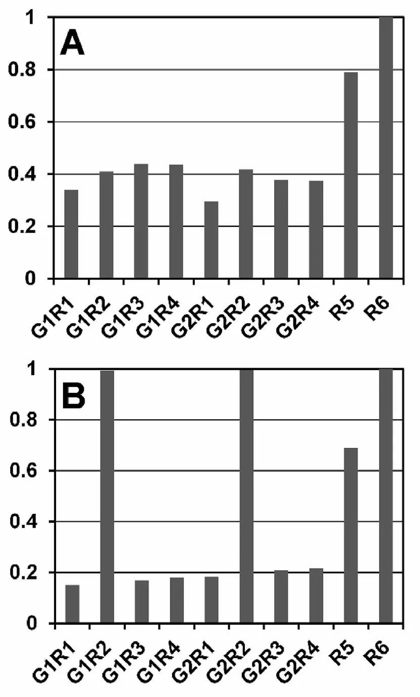
Fig.6.Sums of squared deviations of computed strengthenings from experimental values for examined models normalized to the sum for an R6 model.Afcc alloys,B -bcc alloys.

An analytical approach has been proposed to determine interatomic distance in multicomponent alloys with components having the crystal structure differing from that of the alloy.Based on virtual solvent concept,the methods are also developed to determine atomic size misfit and elastic modulus misfit.Corresponding SSS models were assessed with view point of the best fit to experimental data.The models can be divided into the two groups:G1R1,G1R3,G1R4,G2R1,G2R3,G2R4 models with better agreement and G1R2,G2R2,R5,R6 models with poorer agreement between computed and experimental values.The level of solid solution strengthening for fcc alloys determined in this study is lower as compared to that computed by other authors with a strong underestimation of the friction stress and neglect of the athermal component in the yield point of multicomponent fcc alloys.The G1R1,G2R1,G1R4,and G2R4 models providing the most reliable prediction of SSS may be used to best advantage in multicomponent alloy designing.

Declaration of competing interest

The authors declare that they have no known competing financial interests or personal relationships that could have appeared to influence the work reported in this paper.