Robust optimization design on impeller of mixed-flow pump
, , , , ,
(1.School of Energy and Power Engineering, Jiangsu University, Zhenjiang, Jiangsu 212013, China; 2.School of Materials Science and Engineering, Jiangsu University of Science and Technology, Zhenjiang, Jiangsu 212003, China)
Abstract: To increase the robustness of the optimization solutions of the mixed-flow pump, the impeller was firstly indirectly parameterized based on the 2D blade design theory.Secondly, the robustness of the optimization solution was mathematically defined, and then calculated by Monte Carlo sampling method.Thirdly, the optimization on the mixed-flow pump′s impeller was decomposed into the optimal and robust sub-optimization problems, to maximize the pump head and efficiency and minimize the fluctuation degree of them under varying working conditions at the same time.Fourthly, using response surface model, a surrogate model was established between the optimization objectives and control variables of the shape of the impeller.Finally, based on a multi-objective genetic optimization algorithm, a two-loop iterative optimization process was designed to find the optimal solution with good robustness.Comparing the original and optimized pump, it is found that the internal flow field of the optimized pump has been improved under various operating conditions, the hydraulic performance has been improved consequently, and the range of high efficient zone has also been widened.Besides, with the changing of working conditions, the change trend of the hydraulic performance of the optimized pump becomes gentler, the flow field distribution is more uniform, and the influence degree of the varia-tion of working conditions decreases, and the operating stability of the pump is improved.It is concluded that the robust optimization method proposed in this paper is a reasonable way to optimize the mixed-flow pump, and provides references for optimization problems of other fluid machinery.
Key words: mixed-flow pump;multi-objective genetic optimization;robust optimization;response surface method;2D blade design theory
The mixed-flow pump is widely used in a variety of industrial fields as a good substitution of the centri-fugal pump and axial-pump.However, uncertainties such as the random fluctuation of working conditions will make the optimality and stability of the running pump worse[1-4].Therefore, it is of great engineering value and practical significance to find the optimal pump shape with strong anti-jamming capability from uncertainties.
In existing researches, single-point and multi-point optimizations were mainly used for the mixed-flow pump.WANG, et al[5]used the surrogate model and intelligent optimization algorithm to optimize mixed-flow pumps.WANG, et al[6]optimized a mixed-flow pump under the design operating condition and studied its cavitation performance.JIN, et al[7]applied a weighted-average agent model in a mixed-flow pump optimization, considering the design and off-design operating conditions simultaneously.LIU, et al[8]optimized a mixed-flow pump to obtain the maximum weighted-average hydraulic performance under different working conditions.ZHOU[9]established a three-point hydraulic optimization method to improve pump efficiency under multiple working conditions.In these researches, environmental parameters, optimization va-riables, and objective functions were all predetermined excluding the influence of uncertainties.However, the pump′s performance and operating stability may deterio-rate greatly, once the working conditions fluctuate.
Based on the above issues, this paper aims to develop a robust optimization method for the impeller of a mixed-flow pump to increase its hydraulic performance and working stability at the same time.
1 Original pump
As shown in Fig.1, the pump under investigation is a vertical mixed-flow pump with outlet guide vanes.Its main design specifications are a specific speed ofns=520.17, a flow rate ofQd=4 500 m3/h, and a head ofH=10.34 m at a rotating speed ofn=735 r/min.The main geometric parameters of its impeller are inlet diameterD1=532.58 mm, outlet diameterD2=663.10 mm, blade numberZ1=4.The main geometric parameters of its guide vanes are inlet diameterD3=706.54 mm, outlet diameterD4=641.61 mm, blade numberZ2=6.
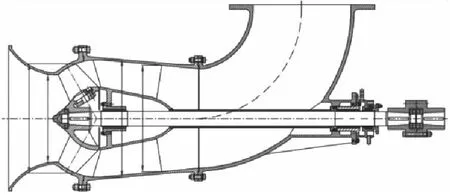
Fig.1 Schematic diagram of mixed-flow pump
Numerical simulations are performed using ANSYS CFX software.From Fig.2, the computational domain consists of four parts including the inlet flow channel, impeller, guide vanes and outlet flow channel.Structured hexahedral grids are generated for the whole computational domain, and grids near the blade surface are refined with localy+less than 5.The total gird number is minimized to 3 132 042 through the grid indepen-dence test[10-13].
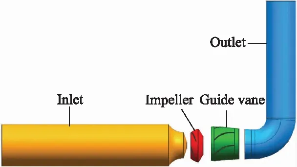
Fig.2 Computational domain
A uniform inlet flow distribution is imposed by setting the flow velocity and a turbulence density of 5%.The outlet is assumed to be a free flow outlet, and the static pressure is set to be 1.01×10⁵Pa here.For the wall boundaries, the non-slip wall boundary condition is imposed.
SSTk-εand standardk-εturbulence models are used for the(0.8-1.0)Qdand(1.0-1.4)Qdworking conditions respectively.The logarithmic wall function is employed to estimate the wall shear stress.The ″Frozen-Rotor-Interface″ model is used to transfer data between the rotor and stator[14-16].
Simulated pump heads and efficiency are compa-red with the tested ones, as shown in Tab.1.It is found that they are in good agreement under all working conditions, and the maximum relative error is less than 5%.

Tab.1 Comparison of the simulated and tested data
Fig.3 shows the simulated static pressure contour on blade surfaces.Fig.4 shows the simulated relative streamlines in the impeller and absolute streamlines in the guide vanes.It is found that with the change of working conditions, the inner flow status in the impel-ler and guide vanes changes, which may aggravate the adverse flow, and lead to unstable flow status and extra energy loss in the original pump.Thus, robust optimization is used to improve its working stability under different working conditions.
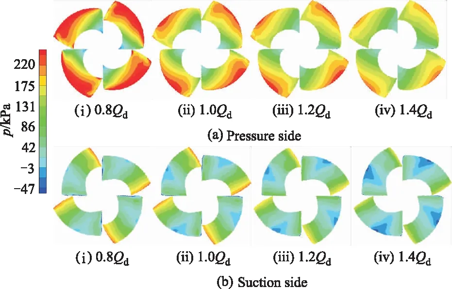
Fig.3 Static pressure contours on blade surfaces

Fig.4 Relative streamlines in impeller and absolute streamlines in guide vanes
2 Blade parameterization
In the 2D blade design theory, a blade profile equation is constructed to build the mathematical relation between the space streamline wrap angle and the meridian streamline length, as shown in Eq.(1).It is also called the motion equation of fluid particle, because it reflects the three-dimensional flow track of particles in the impeller.
(1)
where,θrepresents space streamlinewrap angle;srepresents the meridians treamline length;ωrefers to the rotating speed;rrefers to the radial coordinate;vmrepresents the meridian velocity;vurrefers to the velocity moment.
Using Eq.(1), each space streamline can be decided after the corresponding meridian streamline is given.Then, the blade shape can be decided by mixing all space streamlines and changed by giving the different distribution ofvur.
According to the working principle of the vane pump, the velocity moment difference between the inlet and outlet of the impeller can be calculated by Eq.(2).
(2)
where, Δ(vur)refers to the velocity moment differe-nce;vu1r1andvu2r2are the velocity moment at the inlet and outlet respectively;Hrepresents the pump head;ηhrepresents the hydraulic efficiency;gis the gravitational acceleration.
Then, by introducing a dimensionless quartic po-lynomial functionf(x),vurcan also be described as
vur=vu1r1+f(x)·Δ(vur),
(3)
f(x)=ax4+bx3+cx2+dx+e,
(4)
where,xrepresents the relative meridian streamline length,x=s/s0;s0represents the total meridian strea-mline length;a,b,c,d, andeare coefficients which can be determined by boundary conditions given in Eq.(5).
(5)
In this way, giving differentx1,x2andx3, diffe-rent quartic polynomial functionf(x)is built, and then different distribution ofvuris given, and different blade shape is obtained.
3 Robust optimization
The robustness of feasible solutions is defined as the size of the variable region of objective functions caused by the variation of environmental parameters.It is mathematically defined as
X∈Ω ,i=1, 2, …,m,
(6)
where,mdenotes the number of objective functions;crefers to the environmental parameters;X=(x1,x2, …,xn)represents the optimization variable;nrepresents the dimension of the optimization variable; Ω represents the feasible solution space;F(X)repre-sents the objective function;δrepresents the interfere-nce vector;Bδis the neighborhood with the interference vectorδas the radius.
Since Eq.(6)is difficult to solve, the integral is replaced by summation using Monte Carlo sampling method.Eq.(6)is changed into a new form as
(7)
where,Mindicates the random sampling size in the disturbing neighborhoodBδ;ξjrepresents thej-th sample; and Norm(ξj)refers to the infinite vector norm ofξj.
3.1 Optimization objectives
To improve the headHand hydraulic efficiencyηof the mixed-flow pump, and reduce their fluctuation ranges as far as possible when the flow rate varies between 0.8Qdand 1.4Qd, the optimization problem is divided into two sub-optimization problems, including the optimal sub-optimization problem and the robust sub-optimization problem, as expressed by Eq.(8).
(8)
where,rH(X)andrη(X)are the robustness corresponding to the headH(X)and hydraulic efficiencyη(X)respectively.
Using weight factorsλ1,λ2,λ3andλ4, the two optimization objective of each sub-optimization problem can be synthesized into a single objective as
(9)
Finally, the optimization problem turns into a two-objective maximization problem, in a form as
Maximize[Optimal(X),-Robust(X)].
(10)
To give equal treatment toH(X),η(X),rH(X)andrη(X), weight factorsλ1,λ2,λ3andλ4are all set to be 0.5 here.
3.2 Optimization variable and value range
Parametersx1,x2, andx3constitute a three-dimensional optimization variable as
X=[x1,x2,x3].
(11)
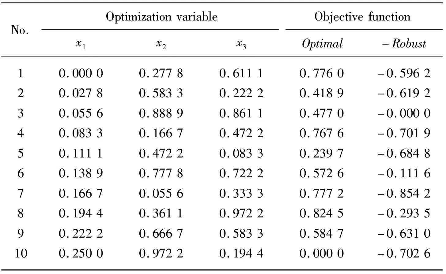
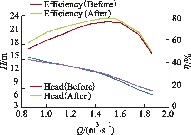
According to the previous research results, the ranges of the optimization variable are set to be 0 According to the value range of the optimization variableX, a uniform design table U37(373)is used to arrange a 3-factor, 37-level initial sample space.Numerical simulations are performed in the whole flow channel of the 37 different pumps under different wor-king conditions.Then,H(X)andη(X)are obtained based on the simulated results.rH(X)andrη(X)are calculated using Eq.(7).Optimal(X)and-Robust(X)are calculated according to Eq.(9).The first 10 groups of data in the initial sample space are listed in Tab.2. Note that, data in Tab.2 are normalized using Eq.(12)to make them vary between 0 and 1. Tab.2 The first 10 groups of data in the initial sample space (12) where,iandjrefers to the index of row and columnyjminandyjmaxrefers to the minimal and maximum sample inj-column, andyjiindicates the sample ini-row andj-column. Based on the first 32 groups of data in the initial sample space, response surface methodology(RSM)is used to construct surrogate models between the optimization variable and objective function. On the Matlab platform, a double-loop iterative optimization process is designed using a multi-objective genetic algorithm, as shown in Fig.5. Fig.5 Flow chart of the robust optimization The first generation of the population is generated randomly and has 200 individuals which are encoded and decoded by the binary encoding and decoding method.Then, the crossover probability, mutation probability and the Pareto-Fraction are set to be 0.8, 0.2 and 0.3, to produce the new generation of the po-pulation by selection, mutation and crossover operations.Thirdly, based on the pre-established RSM surrogate model, the fitness value of each new individual is assigned, and the individuals with high fitness value is selected out and manipulated to produce the next generation of the population by genetic operators.This step will be repeated until the preset maximum iteration number is reached or convergence conditions are satisfied.Finally, the optimal solution is chosen from the last generation of population.Comparisons are made between the RSM predicted and CFD calculated values.If the relative error between them is larger than 3%, the optimal solution will be re-added into the sample space, the surrogate model will be retrained, and the whole optimization process will repeat until the error requirements are met. The optimization is run on the Matlab platform with a 12 core 2.1 GHz workstation, and the convergence conditions are satisfied after 118 steps of iteration which costs about 48 hours.From the Pareto frontier, one optimal solutionX=[x1,x2,x3]=[0.313 1, 0.287 9, 0.001 9]is chosen.Then, nume-rical simulations are carried out on the optimized pump.Finally, based on simulation results, compari-sons are made between the original and optimized pumps. Fig.6 shows the simulatedH-Qandη-Qcurves of the original and optimized pump. Fig.6 Hydraulic performances before and after optimization It is observed that after optimization the efficiency under all working conditions is generally improved,the flow rate corresponding to the highest efficiency point shifts to the left about 0.1Qdand the highest efficiency point changes from 74.11% to 77.07%, with an increase of 2.96%.From theH-Qcurves, it is found that after optimization the head is slightly decreased under the small flow rate, and obviously increased after the flow rate reaches 1.25Qd. To make further comparisons, the width of the high efficiency zoneHEis defined as HE=(Q1-Q2)/QHE, (13) where,QHEis the flow rate corresponding toη=ηmax;Q1andQ2represent the upper and lower flow rate corresponding toη=0.95ηmax. It is found that theHEof the original pump is about 0.265, while theHEof the optimized one is 0.289, with a relative increase of 8.88%.Thus, it can be concluded that the high efficiency area of the mixed-flow pump is widened after optimization. Fig.7 shows the simulated static pressure contour on blade surfaces of the optimized pump. Fig.7 Static pressure contours on the blade surface after optimization Comparing it with Fig.3, it is found that, on the pressure side of the blade surfaces, the area of high pressure zone near the rim decreases after optimization, and the maximum pressure value decreases for the same condition.The small area of low pressure zone near the hub at the inlet also disappears under the 0.8Qdand 1.0Qdconditions, which indicates that the cavitation is weakened at the blade inlet side under the condition of small flow rate.With the increase of flow rate, the static pressure distribution on the optimized blade changes more uniformly, but a local low-pressure zone appears again at the inlet side of the blade when the flow rate reaches 1.4Qd. On the suction side of the blade surfaces, the small area of low pressure zone near the hub at the blade inlet edge disappears after optimization, and the local high pressure zone at the outlet edge is also wea-kened under the flow rate of 0.8Qd, 1.0Qdand 1.2Qd.With the increase of flow rate, although a local low-pressure zone still exists at approximately a third of the blade length near the blade inlet edge, the area of the low-pressure zone is significantly smaller than that be-fore optimization.It indicates that the possibility of ca-vitation is weakened.Based on the above analysis, it can be concluded that the static pressure distribution on the blade surface after robust optimization changes more uniformly with operating parameters. Fig.8 shows the simulated relative streamlines in the impeller and absolute streamlines in the guide vanes of the optimized pump. Fig.8 Relative streamlines in impeller and absolute streamlines in guide vanes after optimization Comparing it with Fig.4, it is found that, under the flow rate of 0.8Qdand 1.0Qd, the stability of flow in the mixed-flow pump has been greatly improved after optimization.The phenomenon of streamline staggering at the outlet of the impeller and inside the guide vane has been weakened.In addition, the number of vortices at the blade inlet decreases, and the vortices size becomes smaller.Under the flow rate of 1.0Qd, the vortex at the trailing edge of the guide vane disappears after optimization.With the increase of flow rate, stream-lines in the impeller and guide vane changes more uniformly after optimization, which indicates that the influence of flow rate fluctuation on adverse flow is weakened. 1)To improve hydraulic performances of the mixed-flow pump and minimize their fluctuation range in case of variations under working conditions, the robust optimization on the impeller of the pump can be decomposed into two sub-optimization problems including the optimal sub-optimization and the robust sub-optimization problem. 2)The uniform test design is a good method to guarantee the reasonable distribution of the initial trai-ning samples for the establishment of the surrogate model.The RSM surrogate model has the smallest overall error and is more suitable for the optimization problem of the mixed-flow pump. 3)Multi-objective genetic optimization algorithm is found to be an efficient way to solve the robust optimization model built for the impeller of the mixed-flow pump.A two-loop iterative optimization method is specially designed to upgrade the sample space and surrogate model with the optimization process, which ensures the rationality of the optimization direction, as well as the acquisition of the global optimal solutions. 4)By comparing the hydraulic performance and internal flow field of the original and optimized pump, it is found that the hydraulic performance, the optimality and stability of the internal flow field of the pump under variable operating conditions are impro-ved, and influence the degree of the variation of ope-rating parameters is weakened.The robust optimization method proposed in this paper proves to be a reasonable way to optimize the mixed-flow pump, and provides references for optimization problems of other fluid machinery.3.3 Initial sample space
3.4 Optimization strategy

4 Results and discussion
4.1 Comparison of hydraulic performance
4.2 Comparison of inner flow field


5 Conclusions

