
A deep energy method for functionally graded porous beams
2021-06-24 13:44ArvinMOJAHEDINMohammadSALAVATITimonRABCZUK
Arvin MOJAHEDIN ,Mohammad SALAVATI ,Timon RABCZUK
1Institute of Structural Mechanics,Bauhaus-Universität Weimar,Weimar 99423,Germany
2Institute of Material Science and Technology,Department of Materials Engineering,Technische Universität Berlin,Berlin 10623,Germany
3Division of Computational Mechanics,Ton Duc Thang University,Ho Chi Minh City,Vietnam
4Faculty of Civil Engineering,Ton Duc Thang University,Ho Chi Minh City,Vietnam
Abstract:We present a deep energy method (DEM) to solve functionally graded porous beams.We use the Euler-Bernoulli assumptions with varying mechanical properties across the thickness.DEM is subsequently developed,and its performance is demonstrated by comparing the analytical solution,which was adopted from our previous work.The proposed method completely eliminates the need of a discretization technique,such as the finite element method,and optimizes the potential energy of the beam to train the neural network.Once the neural network has been trained,the solution is obtained in a very short amount of time.
Key words:Energy-based method;Multilayer perceptron methodology;Functionally graded porous materials;Euler-Bernoulli beam theory
1 Introduction
Porous materials have extensively been used in engineering owing to their remarkable properties,such as their lightweight nature,large specific surface,flexibility,and high resistance to crack propagation.These materials are commonly used in foams,sound absorption,heat insulation,and electrical applications (Altenbach and Ochsner,2010).Functionally graded porous materials (FGPMs) are heterogeneous and have various properties that can be modeled by specific continuous functions(Nguyen et al.,2017;Phung-Van et al.,2017,2019;Thanh et al.,2018,2019).They have been used in mechanical structures such as beams.Numerical methods to analyze such beams include the finite element method (FEM),Rayleigh-Ritz method,finite difference method,and boundary element method.Numerous studies have examined the behavior of functionally graded material (FGM) beams using different theories.For example,Sankar (2001) analyzed a functionally graded (FG) beam imposed on transverse loads,in which the obtained displacement and stress fields of the FG beam were compared with homogeneous beams.Li et al.(2002) analyzed buckling and post buckling behavior of elastic rods subjected to thermal loads and solved the nonlinear equilibrium equations of Euler-Bernoulli beams using the shooting method.Mojahedin et al.(2018) presented an exact solution of functionally graded porous (FGP) beams under in-plane thermal loading condition using an energy-based method assuming a power-law composition for the constituents and considering both saturated and unsaturated pores.Galeban et al.(2016) studied the free vibration of FG thin beams composed of saturated porous materials.The nonlinear equations of motion were derived using a variational formulation based on the Euler-Bernoulli beam theory.The natural frequencies of the FGPM beam were analytically obtained for different boundary conditions.Moreover,they quantified the effects of poroelastic parameters and pore compressibility on natural frequencies.Chen et al.(2016) investigated the free and forced vibration characteristics of FGPM Timoshenko beams subjected to different loads,including a harmonic point load,impulsive point load,and moving load with constant velocity.The equation of motion was discretized using FEM(using the commercial software package ANSYS) in space,and the Newmark-βmethod was employed for time discretization.Alshorbagy et al.(2011) used FEM to discretize the FGM beam.The large displacement behavior of tapered cantilever beams composed of FG materials under end force conditions was investigated by Nguyen(2014).Chakraverty and Pradhan(2016) analyzed the free vibration of beams composed of FGMs under different boundary conditions based on classical and first-order shear deformation beam theories.They obtained the governing equations using the Rayleigh-Ritz method.Ghannadpour et al.(2013)investigated the bending,buckling,and vibration of nonlocal Euler beams.They used the Ritz method to analyze nonlocal beams under four classical boundary conditions.Their results demonstrated the effectiveness of the Ritz method for modeling nonlocal beams.
Solving differential equations using deep learning methods includes the advantages of lower computational cost,easy training,and parallel computing(Tran-Ngoc et al.,2019;Khatir et al.,2020;Nguyen-Le et al.,2020).Numerous studies have used deep learning solutions for partial differential equations(PDEs).Liu et al.(2019) solved differential equations based on a multilayer feedforward neural network.They presented an neural network model with a combination of a boundary term and multilayer feedforward network.This model improved the accuracy and satisfied the boundary conditions.Nabian and Meidani (2018) used a deep learning approach to solve ordinary differential equation (ODE)/PDE of diffusion and heat conduction problems.They approximated the problems by applying the variation of parameters of a residual neural network.Anitescu et al.(2019) solved second-order boundary value problems using a feedforward fully connected (FC) deep network and adaptive collocation strategy.They used an adaptive approach to select collocation points based on the residual value of the previous training steps.This method improved the robustness of the collocation method in cases of nonsmooth regions.
Sirignano and Spiliopoulos (2018) considered Hamilton-Jacobi-Bellman PDE and Burgers’ equation by approximating a deep neural network(DNN)solution.They presented an algorithm that combined the Galerkin method and deep learning neural network.The deep learning neural network was trained to satisfy the differential operator and initial and boundary conditions.Shirvany et al.(2009)obtained PDE and ODE equation solutions using multilayer perceptron (MLP) methods.The algorithm was validated by analytical solutions and two well-known numerical methods,i.e.,Runge-Kutta method and FEM.The algorithm results showed high accuracy,fast convergence,and low memory usage to solve differential equations.Lagaris et al.(1998) studied the deep learning method to solve initial and boundary value problems.Their scheme used adjustable parameters(weights)in the network only for PDEs,and boundary conditions were not updated during the training.The results of the method were compared with solutions obtained using the Galerkin FEM for several cases of PDEs.Weinan and Yu (2018) used the deep learning method to numerically solve variational problems,particularly those occurring from PDEs.They used variational energy as an objective function to optimize the neural network.They demonstrated that this approach yields appealing visual results,and a short empirical convergence analysis was performed.
In this study,we propose a deep energy method(DEM)for FGP beams based on the Euler-Bernoulli theory to solve the nonlinear strain-displacement relations.Therefore,a loss function,which is the potential energy of the system,is minimized using the Adam optimizer.Boundary conditions are imposed using the penalty method.The method is implemented in PyTorch.
2 Deep energy method
DNN predicts the nonlinear relationship between input and output variables.We use a feedforward DNN by employing the deep learning technique (Fig.1).Feedforward networks comprise an input (x) layer,hidden layers (H),and an output layer (Y(x)).At a given layer,the input from the previous layer is mapped to a neuron through the corresponding weights and biases.MLP employs some form of gradient descent for training(updating the weights and bias) using the backward propagation algorithm,in which large gradients indicate a fast training process.During training,once the loss function is minimized,the weights(θ)and biases(b)are stored as a set of connections.
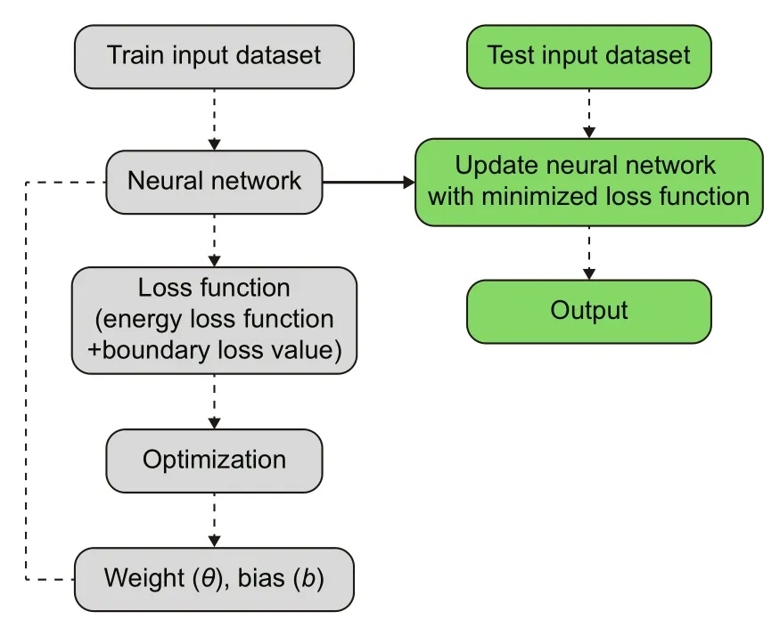
Fig.1 General supervised learning algorithm
2.1 Neural network architecture
The network architecture is essential.In this study,it is constructed by batching three blocks,in which each block comprises two FC linear transformations,two nonlinear activation functions (AFs),and a residual connection (Fig.2).The output of each block is vectors in Rm.For a given input vectorxxxj=(x1,x2,...,xn),the output of the network can be expressed as(Weinan and Yu,2018):
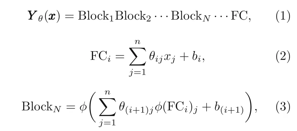
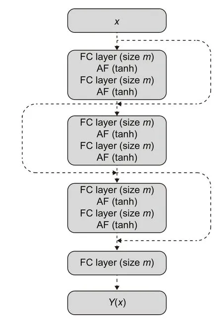
Fig.2 DNN network with three blocks and a linear output layer (FC).Each block consists of two FC layers and two nonlinear AFs
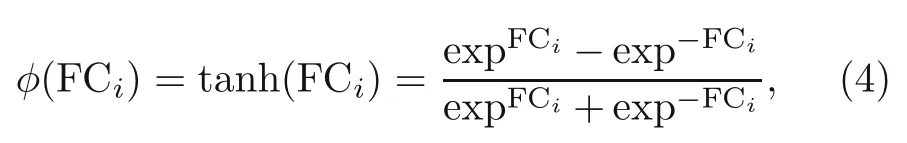
whereφis the nonlinear AF,nthe number of training points,FCitheith FC layer,and BlockNtheNth output block (Goodfellow et al.,2016).The number of updated parameters (Pa) in each layer is calculated as
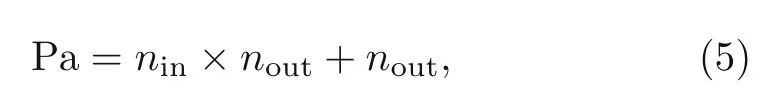
whereninandnoutdenote the number of neurons in sequentially connected layers.
2.2 Energy method and loss function
Let us consider a FGP beam with a rectangular cross section under distributed loading condition.The graded properties are assumed to vary through the direction of the thickness (z-axis).The length,width,and height of the beam are denoted byl,s,andh,respectively(Fig.3).
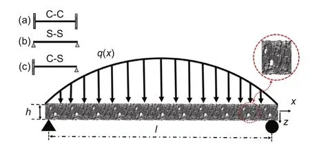
Fig.3 Geometry system of an FGPM beam under external distributed loading condition q(x),where(a),(b),and (c) denote the clamped-clamped (C-C),simply-simply (S-S),and clamped-simply (C-S) supported boundary conditions,respectively
2.2.1 Functionally graded Euler beam
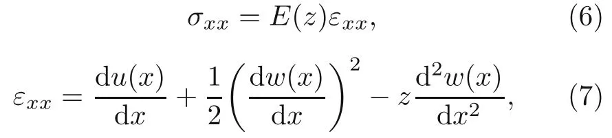
Let us consider the Euler-Bernoulli theory.The stress-strain (σ-ε) relation and kinematic equations are given as whereu(x) andw(x) denote the displacements inx(axial) andzdirections,respectively.The porous material has a nonlinear symmetric porosity distribution along the thickness.The elastic modulusEis assumed to be a function ofz(Galeban et al.,2016):
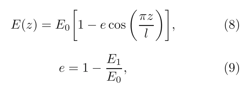
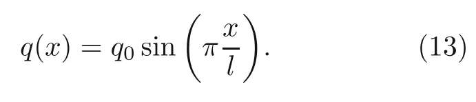
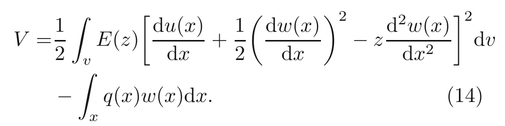
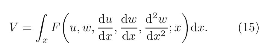
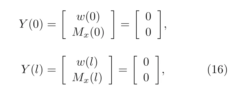
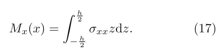
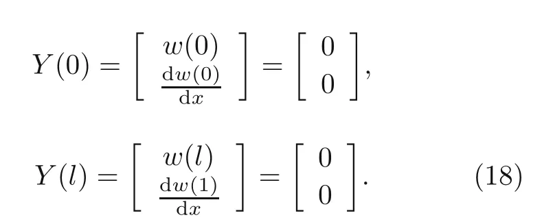
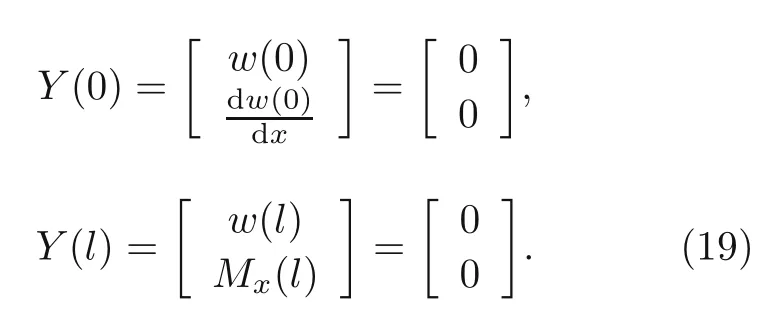
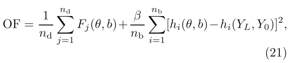
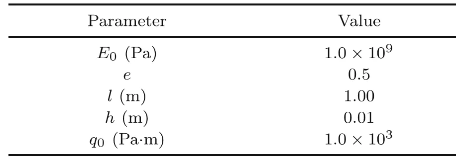
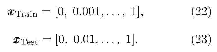
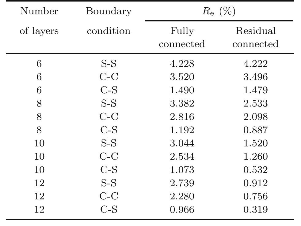
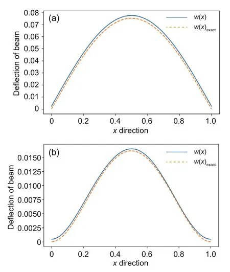
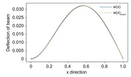
whereeis the beam porosity coefficient(0 2.2.2 Variation formulation The total potential energyVis the sum of strain energyUand the potential energy of the applied loadW: wherevis the volume,andq(x) indicates the distributed load.In our examples,we consider distributed load of the form By substituting Eqs.(6) and (7) into Eq.(11),the following expression forVis obtained: Integrating with respect toz(−h/2 toh/2) andy(−s/2 tos/2)yields the total potential energy: 2.2.3 Boundary conditions We considered three types of boundary conditions:simply-simply supported,clamped-clamped,and clamped-simply supported(Fig.3). 1.Simply-simply support where the beam moment is expressed as stress variation through the thickness based on the Euler-Bernoulli beam theory: 2.Clamped-clamped support 3.Clamped-simply support 2.2.4 Loss function and optimization DEM is based on minimizing a loss function,which comprises Eq.(15) and boundary terms(Eqs.(16)–(19)),guaranteeing the fulfillment of essential boundary conditions: whereh(YL,Y0) corresponds to the functional boundary conditions.Substituting the fulln-layer network Eq.(1) into Eq.(20) yields the loss function(OF) in terms of the weights(θ) and biases(b).Essential boundary conditions are imposed with the penalty method,as previously mentioned.Using the rectangle rule to evaluate the integrals in Eq.(20)finally yields the following objective function: wherendandnbare the numbers of collocation points in the domain and at the(essential)boundary,respectively,andβis the penalty parameter.The second term on the right hand side of Eq.(21)corresponds to the sum of squared distances between the actual/target values (hi(YL,Y0)) refer to Eqs.(16)–(19)and predicted(hi(θ,b))values. The optimization process minimizes the objective function with respect to weights (θ) and biases(b).We used the Adam optimizer (Kingma and Jimmy,2015),which is based on the stochastic gradient descent method and readily available in PyTorch. Let us consider the FGP beam with three types of boundary conditions (Fig.3).The material parameters are listed in Table 1. Table 1 FGPM beam properties To design an effective network,we stacked six FC layers with skip/residual connections linked at their end with pure FC linear layer (Fig.2).The training dataset comprises equally distanced 1000 points on the solution domain,while the testing dataset comprises different 100 points: The number of each hidden layer(nout)includes 150 neurons,and the output layers include a dataset(www),which equals the number of input dataset (n).During training,the updating rate of weights refers to the step size or learning rate (η),which is an important hyper-parameter when configuring the neural network.It controls the pace at which the model is adapted to the problem.We select a learning rate ofη=0.015 with 100 training approaches. The residual network is often easier to optimize than the FC network.The block-to-block skipping simplifies the network’s performance.By increasing the impact of gradients,the learning speed is increased,which leads to better results because there are fewer layers to propagate in the initial training stages.The relative errors obtained from this network architecture and FC neural network are compared in Table 2.By increasing the number of hidden layers and using a deeper network,the relative errors in the residual network decrease.The relative error(Re)is defined as Table 2 Relative error of FC and residual networks wherew(x)exactandw(x)are the exact and predicted solutions of the FGP beam’s deflection,respectively. Fig.4 compares the solution of DEM with the exact solution for clamped-clamped and simplysimply boundary conditions.Notably,the accuracy can be improved by increasing the number of blocks in Fig.2 and the size of the input dataset.Fig.5 compares the predicted and exact solutions for the clamped-simply boundary condition.Changing the boundary conditions insignificantly affects the accuracy. Fig.4 Comparison of the exact (w(x)exact) (Reddy,2017) and our predicted (w(x)) solution results of residual network with six layers for simply-simply (a)and clamped-clamped (b) boundary conditions Fig.5 Comparison of the exact (w(x)exact) (Reddy,2017) and our predicted (w(x)) solution results of residual network with six layers for clamped-simply boundary condition We proposed DEM to study the bending behavior of porous Euler-Bernoulli beams under various boundary conditions and adopted an analytical solution from our previous work to compare the performance of our method.DEM only requires the definition of the potential energy of the system and eliminates the need of a classical discretization,such as finite element method.It can be easily implemented in standard open-source tools such as PyTorch.The objective function,which corresponds to the potential energy of the system plus a term to impose essential boundary conditions,is minimized using the Adam optimizer.We employed tanh as the activation function and determined that an increase in the number of input neurons and blocks in the network structure up to a certain point yields results with acceptable precision and convergence to the exact solution.However,at a certain point,a further increase causes overfitting.Moreover,we determined that the residual network is easier to optimize (with lower computational cost) compared with the fully connected network. Contributors Timon RABCZUK devised the project,verified the computational process,and contributed to the final version of the manuscript.Mohammad SALAVATI contributed to the simulation process.Arvin MOJAHEDIN worked out the technical details,performed the computational calculations,and wrote the manuscript. Conflict of interest Arvin MOJAHEDIN,Mohammad SALAVATI,and Timon RABCZUK declare that they have no conflict of interest.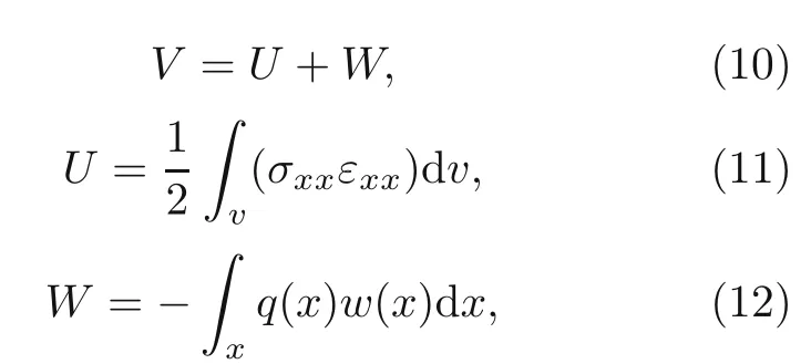

3 Results and discussion
4 Summary and conclusions
 Journal of Zhejiang University-Science A(Applied Physics & Engineering)2021年6期
- Journal of Zhejiang University-Science A(Applied Physics & Engineering)的其它文章
- Optimizing the neural network hyperparameters utilizing genetic algorithm
- Prediction of the load-carrying capacity of reinforced concrete connections under post-earthquake fire
- Damage detection in steel plates using feed-forward neural network coupled with hybrid particle swarm optimization and gravitational search algorithm*