Optimizing the neural network hyperparameters utilizing genetic algorithm

Saeid NIKBAKHT ,Cosmin ANITESCU ,Timon RABCZUK

1Division of Computational Mechanics,Ton Duc Thang University,Ho Chi Minh City,Vietnam

2Faculty of Civil Engineering,Ton Duc Thang University,Ho Chi Minh City,Vietnam

3Institute of Structural Mechanics,Bauhaus-Universität Weimar,Weimar 99423,Germany

Abstract:Neural networks (NNs),as one of the most robust and efficient machine learning methods,have been commonly used in solving several problems.However,choosing proper hyperparameters (e.g.the numbers of layers and neurons in each layer) has a significant influence on the accuracy of these methods.Therefore,a considerable number of studies have been carried out to optimize the NN hyperparameters.In this study,the genetic algorithm is applied to NN to find the optimal hyperparameters.Thus,the deep energy method,which contains a deep neural network,is applied first on a Timoshenko beam and a plate with a hole.Subsequently,the numbers of hidden layers,integration points,and neurons in each layer are optimized to reach the highest accuracy to predict the stress distribution through these structures.Thus,applying the proper optimization method on NN leads to significant increase in the NN prediction accuracy after conducting the optimization in various examples.

Key words:Machine learning;Neural network (NN);Hyperparameters;Genetic algorithm

1 Introduction

During the past few years,machine learning(ML) algorithms have attracted scientists’attention in solving various problems (e.g.image recognition,search engine result refining,email spam detection,and malware filtering) due to considerable advances in the capacity of computers.Neural networks (NNs) are widely used in many ML applications due to their capability of solving various practical problems (e.g.speech processing (Nassif et al.,2019),computer vision (Alhichri et al.,2018),and weather forecasting (Dalto et al.,2015)).Similar to other scientific fields,mechanical engineering has also been influenced by this novel methodology.Moreover,numerous studies using NN have been carried out.Nguyen-Thanh et al.(2019)implemented a deep neural network(DNN)method to find the stress and displacement distributions through mechanical structures such as 2D and 3D cantilever beams under bending and twisting T-shaped bars.The total potential energy of the system was considered as the loss function which was minimized using Adam and limited-memory Broyden-Fletcher-Goldfarb-Shanno(L-BFGS) optimization methods.The boundary conditions were also taken into account to reach the proper network parameters through the backpropagation procedure.The authors referred to this strategy of solving mechanical problems as the deep energy method(DEM).Moreover,the DEM computational time is significantly higher compared with the classical numerical methods such as the finite element method (FEM).However,using DEM gives accurate solutions much faster than FEM when the network is trained for various types of boundary conditions.Samaniego et al.(2020)also used DEM for solving several mechanical problems(e.g.phase-field modeling of fracture,piezoelectric cantilever beam,and Kirchhoffplate under bending).This method was also compared with the collocation method and demonstrated the DEM advantage in solving partial differential equations which are capable of using the variational format of the boundary value problem instead of the strong format.Other NN applications for analyzing mechanical problems can be found in(Najafi et al.,2018;Goswami et al.,2020;Shamshirband et al.,2020).

The accuracy and convergence of the different types of NN highly depend on hyperparameters(e.g.the numbers of hidden layers and neurons in each layer),which are often arbitrarily chosen.In the past few years,several studies have been done on optimizing the NN hyperparameters.Yu and Zhu(2003)presented a comprehensive review in this field in which the performance of various methods in optimizing the NN hyperparameters was compared and discussed.Three approaches exist to mainly find the best hyperparameters.The grid search (GS) is the first method in which all the combinations of different hyperparameters are evaluated.Moreover,the combination with the lowest cost function or the highest fitness is introduced as the best set of hyperparameters.In addition,other useful application of deep learning was shown by Kaur et al.(2020)to classify and predict people who have Parkinson’s disease.Different voice features of the patients were gathered into a dataset and a DNN was applied to it.Furthermore,the authors attempted to find the best hyperparameters of their approach using GS.They finally managed to increase the overall and mean prediction accuracies of their model up to 89.2%and 91.7%,respectively.However,using GS requires a vast amount of computations to obtain the absolute best network architecture.Therefore,it is not an effi-cient method.Moreover,the so-called random search(RS) method was devised to avoid this exhaustive search through all possible combinations of different hyperparameters (Bergstra et al.,2012;Torres et al.,2019).An arbitrary number of hyperparameter combinations are randomly chosen in this approach,and the best result is introduced as the optimal set of hyperparameters.Although using RS may not lead to the highest fitness or lowest cost function,its computational time is considerably lower than GS.Consequently,Jo et al.(2019)employed the artificial NN(ANN)to estimate the exhaust gas recirculationlow pressure (EGR-LP) rate in turbocharged gasoline direct injection(GDI)engines and attempted to improve the hyperparameters of their approach using three methods of RS,tree-structured Parzen estimator,and hyperparameter optimization via radial basis function and dynamic coordinate search(HORD).These authors compared the mentioned algorithms and proved that HORD,with a validation performance of nearly 99%,was capable of more accurately predicting the EGR-LP rate.Moreover,Motta et al.(2020) applied a convolutional neural network(CNN) on a dataset with 8700 images containing 7500 mosquito images to classify mosquitoes which cause specific disease and distinguish the difference between them and other types of insects.However,the authors used a data augmentation strategy to increase the size of training and test datasets because not enough data were available to carry out this study.Subsequently,the RS and GS methods were implemented for tuning the hyperparameters of the used CNN,which managed to increase the accuracy of image recognition from 76%to 93%.

Searching blindly through the domain of the hyperparameter is the main disadvantage of the RS method.However,metaheuristic algorithms such as genetic algorithm (GA) can overcome this problem.Therefore,the combinations of hyperparameters with the best results in each step are saved.Subsequently,the new sets of hyperparameters in the next step are generated by combining the hyperparameters of the previous step.Thus,the search process is not blind and the possibility of reaching the optimal result is higher than RS.A comparison study on the accuracy and computational time between GS,RS,and GA was reported by Liashchynskyi and Liashchynskyi (2019).According to their revealed results on the CIFAR-10 classification dataset,GA outperformed the other mentioned methods.

Two characteristics exist in every GA approach.The first one,referred to as diversification or exploration,is the capability of the algorithm to represent a general overview of the entire solution domain and distinguish the areas which have the potential of producing better results.This feature helps the optimization process not to waste time on areas in which the chance of achieving the optimum result is low.The second one,intensification or exploitation,is defined as intensifying the search through the areas with promising results and trying to find the best possible solution in those fractions of the solution domain.These qualities are the main advantages of GA over RS which signifies that GA is a more efficient method.As a result,a decent number of studies on the application of GA in optimizing the NN hyperparameters have been carried out.Consequently,image recognition research on the images of four different types of leukocytes(white blood cells)was conducted by Bani-Hani et al.(2018) with nearly 10 000 and 2500 training and test data,respectively.The authors improved their results by combining CNN with GA to find the optimal CNN parameters,leading to more accurate image classification.In another image recognition study carried out by Loussaief and Abdelkrim(2018),the numbers of convolutional layers and filters,as well as their sizes in each layer,were optimized using GA.They managed to increase the classification accuracy of the CNN from 90% to>98%.Wei and You (2019) adopted GA to improve the fitness of the modified national institute of standards and technology (MNIST) image recognition problem and managed to increase the prediction accuracy from 98.10% to 98.84%.In addition,the authors developed a two-point fusion intermediate crossover and adaptive mutation to optimize the hyperparameters of the fully connected NN.The adaptive mutation maintained the scale of variation at the beginning of the evolution process,and the diversity of the population gradually decreased as the model evolved.This helped the GA process to explore the domain properly and to boost local fine-tuning.Moreover,Wicaksono et al.(2018)completely discussed the benefits of GA over GS in comprehensive research on hyperparameter optimization of different ML algorithms.Consequently,this study revealed that GA could be almost as accurate as GS but could significantly decrease the computational costs,particularly when the solution domain is quite large.The authors applied this metaheuristic algorithm on several ML approaches (e.g.support vector machine (SVM),random forest(RF),K-nearest neighbor,and adaptive boosting).In addition,the reduction in computational time of these methods was up to 85%.

The process of backpropagation in NNs causes two problems,i.e.first,converging into undesirable local minima,and second,the constant scheduled learning rate which can slow down convergence.To overcome these problems,Kanada (2016) used the learning rate optimizing genetic backpropagation (LOG-BP) method in which GA is combined with the process of backpropagation in a CNN image recognition study.Thus,the weights and biases along with the learning rate in each epoch are acting as chromosomes,and the learning rate is mutated when the best weights and biases are found.Subsequently,the optimum chromosomes are passed to the next epoch.According to MNIST benchmarking,LOG-BP showed better performance compared to the conventional stochastic gradient descent methods.Moreover,another contribution to the optimization of hyperparameters in a CNN-based study was done by Guo et al.(2019) who used the Tabu-GA method for image recognition of MNIST and Flower-5 datasets.The authors demonstrated that using a Tabu list to avoid evaluating repetitive chromosomes has a significant influence on the optimal results because their method finally outperformed the common methods such as RS and Bayesian optimization while the computational costs of Tabu-GA were 50%less.

Other metaheuristic algorithms are also used to improve the accuracy and efficiency of problems dealing with NN.Junior and Yen(2019)used the particle swarm optimization(PSO)to find the best hyperparameters which yield the least computational costs and best accuracy of image classification employing CNN.Three groups of PSO,CNN architecture initialization,and CNN training parameters were controlled in this study to find the CNN with the highest fitness in classifying the images of the MNIST dataset.The authors finally showed the superiority of their method(called psoCNN)over other methods,and only 30 particles and 20 iterations were found to be enough to reach accurate results comparable to other hyperparameter optimization approaches.Furthermore,two metaheuristic algorithms (firefly and tree growth algorithms) were developed by Bacanin et al.(2020)to optimize the hyperparameters of a CNN in an image recognition approach.The authors manipulated these algorithms to enhance their exploration-exploitation balance and proved the outperformance of their algorithm over their conventional counterparts in terms of robustness and classification accuracy.All the experiments were conducted on an MNIST dataset,and the numbers of convolutional layers,filters,and fully connected layers,and the size of the filters acted as the design variables in this study.In a novel CNN-based approach,ul Hassan et al.(2018)attempted to classify the images of MNIST and neuromorphic MNIST datasets into two groups of good and bad quality images without understanding the image content.Subsequently,the authors optimized the hyperparameters of their classification problem implementing a hyperheuristic approach that improved the CNN learning performance.The most beneficial feature of the applied optimization method was the capability of improving the learning process when the training dataset is not sufficiently large.

2 Mathematical formulation

2.1 Principle of minimum potential energy

The potential energy of a mechanical system(ε)under traction (tN) and body force (f) is obtained as follows:

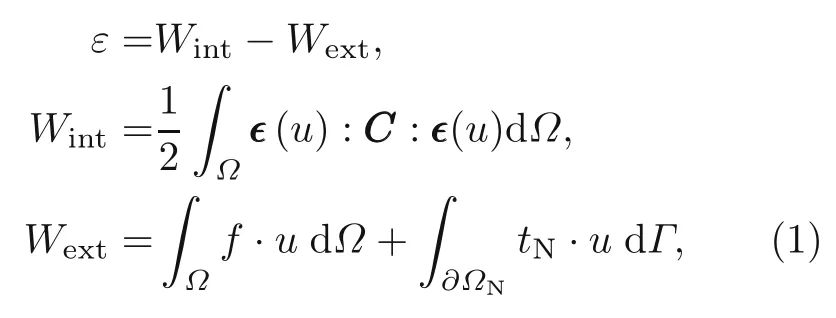
whereWintandWextare the stored elastic strain energy and the work of external force,respectively.Cand∊represent the stiffness matrix and strain tensor which is a function of displacements(u).Note that the integrals related to stored elastic energy and body force are obtained on the whole domain (Ω),while the integral of traction force is calculated on the surface on which the traction is imposed (Γ).In addition,the Drichlet and Neumann boundary conditions are imposed as

whereΩDandΩNare the Drichlet and Neumann boundaries,and ¯uandtNindicate the prescribed values on these boundaries,respectively.σandNNNdenote the first Piola-Kirchhoffstress tensor and outward unit normal vector,respectively.Moreover,the principle of minimum potential energy states that the total potential energy should be minimized to reach the stationary conditions.

2.2 Deep neural network

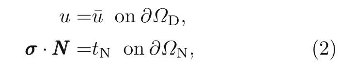
ANNs are widely used to solve various problems(e.g.speech recognition and image classification).These methods are capable of classifying massive data.Given an input vectorxinto a simple NN,the output vectorucan be calculated as

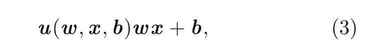
wherewandbare the network parameters called weights and biases,respectively.These network parameters are randomly chosen,and they are modified through the backpropagation process by minimizing a loss function that is related to the total energy of the system in the application of this study.In addition,a DNN is an ANN with more than one hidden layer.The output of the DNN is calculated as

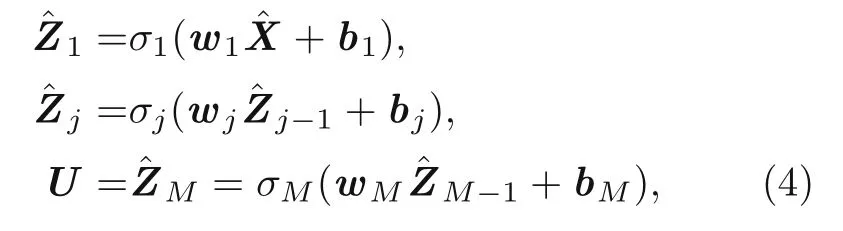
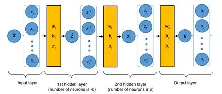
Fig.1 A schematic of a two-layered DNN (is the output vector at the training point)

The activation function introduces nonlinearity to the model.Without an activation function,the model is a linear regression model and is not capable of analyzing complicated input data.The activation function is a linear or nonlinear function acting as a mathematical gate between the adjacent layers so that the output of each layer goes through an activation function to the next layer.Therefore,the hyperparameters affect the convergence rate and accuracy of the model to a great extent.In addition,the activation function related to the output layer should be a linear function to reproduce unrestricted outputs.Common activation functions include Sigmoid,tanh,rectified linear unit (ReLU),and ReLU2(Fig.2).

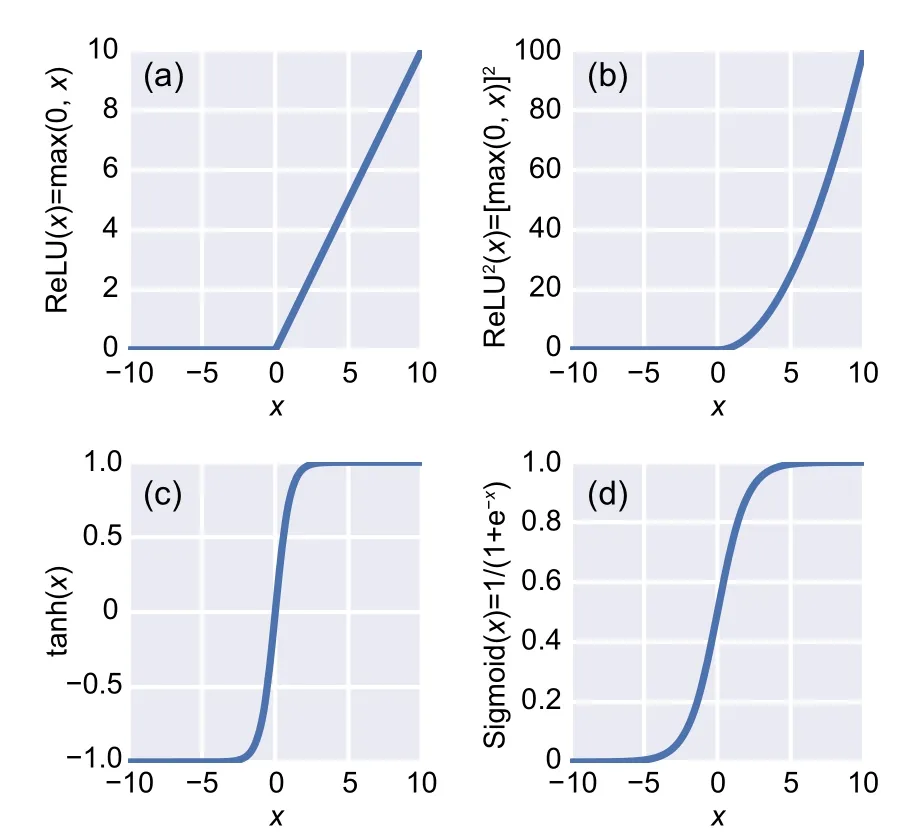
Fig.2 Nonlinear activation functions:(a) ReLU;(b)ReLU2;(c) tanh;(d) Sigmoid

2.3 Deep energy method

DEM is a novel and simple machine learningbased method of solving partial differential equations(or energy problems).It is based on combining the principle of minimum potential energy with the DNN concept.Therefore,integration points are placed in the domain and along the boundary.Subsequently,the total energy of the system is considered as the loss function of the applied DNN.It is minimized through training the model for a certain number of epochs.This process is illustrated in Fig.3.

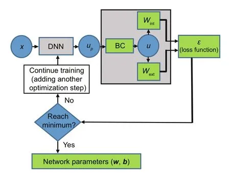
Fig.3 A schematic of DEM procedure(BC represents boundary condition)

After finding the modified network parameters (weights and biases),new sets of integration points are generated as the test data.In addition,the displacements related to the test data are predicted.Finding the derivatives of the displacements yields the strain tensor,and the stress distribution through the structure is calculated using the constitutive equations.Several optimizers including the Adam optimizer followed by the LBFGS method with boundary constraints(L-BFGSB method) were tested.The network is trained for a certain number of iterations using Adam optimizer.Subsequently,the L-BFGS-B method is used for training the network to reach a certain accuracy.The desired accuracy in this study is reached when the discrepancy between the loss functions obtained through successive iterations is<10−8.

3 Genetic algorithm

In this section,the hyperparameters of the NN implemented in DEM are optimized using GA.The relativeL2error associated with the total strain energy of the system is taken as the objective function to be minimized.Conversely,the numbers of neurons in each layer or the number of integration points are considered as the design variables.Three basic steps exist when solving a minimization problem using GA.In the first step,a population called parents is selected among all the possible solutions(chromosomes)of the desired problem.In the second step,two secondary populations called offsprings and mutants are generated through crossover and mutation procedures,respectively.In the third step,all the populations are merged and sorted according to their objective functions.Finally,a certain number of the best populations are chosen and the rest are truncated.This procedure is repeated for a certain number of iterations to find better optimal results.

3.1 GA initialization

The GA process begins with randomly choosing a certain number of chromosomes (Pinit) in the solution domain.This primary population is updated through the rest of the GA procedure by adding a certain number of offsprings and mutants.

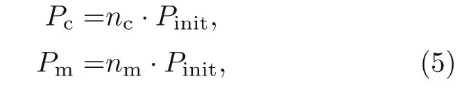
wherencandnmdetermine the fraction of initial population chosen for crossover and mutation,respectively.PcandPmdenote the population obtained by the crossover and mutation processes,respectively.Moreover,the size ofPinitremains constant after each iteration by truncating the worst chromosomes.The number of truncated chromosomes in each iteration is equal tonc+nm.

3.2 Crossover

In the crossover process,a pair of parents is chosen to generate a pair of offsprings.These new chromosomes are calculated by combining the two parents as

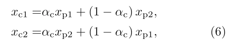
wherexc1andxc2are the offsprings andxp1andxp2are the parents.αcis a parameter randomly chosen between−γand 1+γwhich controls the similarity rate between the parents and offsprings,respectively.In addition,γis another arbitrary parameter that helps the search through the solution domain to cover larger areas,which could result in better GA exploration and better final results convergence.

3.3 Mutation

The crossover process in the GA may lead to local minima.Thus,another strategy is suggested to overcome this issue.In this strategy,called mutation,one parent is selected to generate a new chromosome called mutant by randomly changing one of the components of the selected parent as

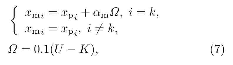
whereαmis a parameter between 0 and 1 which defines the similarity level between the parent and mutant.In addition,UandKare the upper and lower bounds of the number of neurons chosen for the layers of NN,respectively.The numbers of neurons in the offsprings and mutants are also controlled to be betweenKandU.

3.4 Tabu list

A huge number of new populations are generated during the crossover and mutation procedures.In addition,a major number of repetitive chromosomes exist after these processes which results in extra useless computations.Furthermore,having a repetitive population could lead to inefficiency and deprive the GA of properly searching the domain.Therefore,all the evaluated chromosomes are saved in a Tabu list,and this list is updated through the complete process of optimization.In each GA step,all the new generated chromosomes are compared with the Tabu list.Thus,it is discarded if it has already been evaluated.Consequently,a large number of extra computations are avoided and the search process is more effectively conducted with the Tabu list.Moreover,Fig.4 shows the complete procedure of implementing GA on DEM.

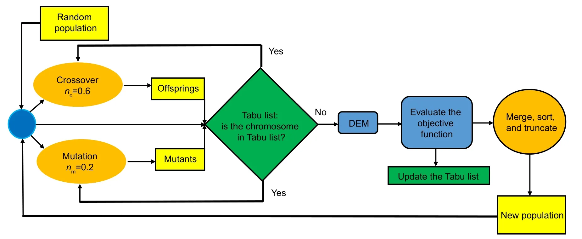
Fig.4 Process of GA in optimizing the network DEM hyperparameters

The GA parameters,mainly the crossover and mutation probabilities,influence the optimal results and the convergence rate.These parameters are differently chosen for the size of the solution domain and the nature of the problem.Too little mutation rates lead to local minima while too large mutation rates hinder the process of finding the best solution and therefore decrease the convergence rate.To avoid local minima,a large mutation rate(0.2)is chosen.Thus,four new chromosomes are generated through the mutation procedure in every GA iteration.Moreover,the crossover probability should be large(>0.5)to more intensely search the specific area with optimum results.Therefore,this parameter resulted in a 0.6 probability.Consequently,12 new chromosomes are produced through the crossover procedure during each iteration.The GA parameters used in this study are presented in Table 1.

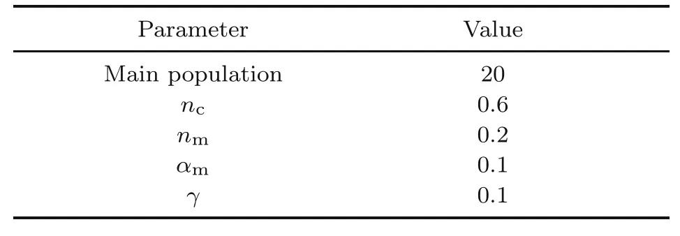
Table 1 GA parameters

4 Results and discussion

This section presents the results related to the stress distribution of a Timoshenko beam and a plate with a hole obtained by DEM with a three-layered NN each containing 30 neurons.Subsequently,the best optimizer and activation function are found by comparing the results of DEM containing various optimizers and activation functions.The DEM network architecture is afterward optimized considering different sets of integration points as the input data.The stress distribution through both aforementioned structures is calculated using DEM with the optimized hyperparameters.Moreover,the results are compared with those of analytical solution and DEM with predefined network architecture to show the impact of hyperparameter optimization on the accuracy of predicting output results.Another example is shown by the optimization of the number of integration points while the network architecture is fixed.Finally,the convergences of the resultsfor training and test datasets are compared to show whether overfitting has occurred or not.

4.1 DEM with predefined network hyperparameters

4.1.1 Timoshenko beam

This section used DEM for estimating the stress and displacement distributions of a Timoshenko beam under point loading.The results are compared with those of the study carried out by Augardee and Deeks(2008).According to this work,the exact displacement and stresses through these beams can be calculated as

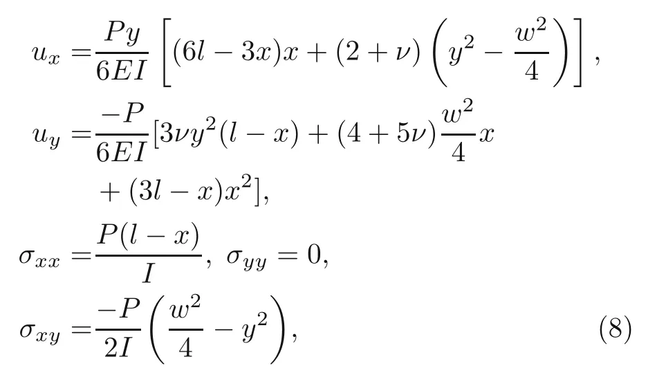
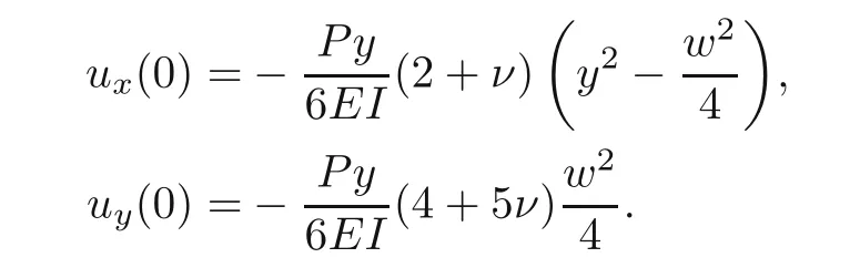
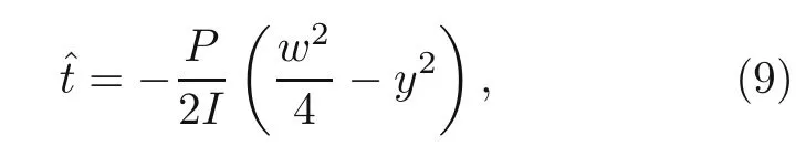
whereP,l,I,andware the magnitude of point load,length of the beam,the second moment of area of the cross-section,and width of the beam,respectively.In addition,Eandνdefine the elastic modulus and Poisson’s ratio,respectively.The loading at the end of the beam must be imposed as a parabolic varying shear force to provide the stability of this bending problem.Moreover,the essential boundary conditions at the fixed end must be satisfied according to the aforementioned displacement field through the beam.Therefore,the boundary conditions of the beam should be satisfied as follows:

The Drischlet boundary conditions:

The Neumann boundary conditions:

The coordinate system of the cantilever beam is demonstrated in Fig.5.

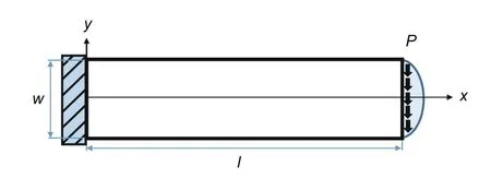
Fig.5 Coordinate system of the cantilever Timoshenko beam problem

This study considered the total energy of the system (strain energy and energy of the external forces)as the loss function of DEM to find the stress and displacement distributions of the Timoshenko beam.In the first step,the interior and boundary integration points and weights are generated using the non-uniform rational B-spline (NURBS) functions and Gaussian quadrature integration method.Next,a DNN with three layers each containing 30 neurons is constructed.Consequently,the Adam optimizer followed by L-BFGS-B are taken as the optimization methods to minimize the loss function,while ReLU2acted as the activation function.Finally,the network is trained,and the predicted displacement and stress distributions of these loaded beams are calculated.After comparing the predicted displacements with the exact solution,relativeL2errors associated with displacements and energy of the beam under the mentioned load are calculated to show the DEM accuracy:

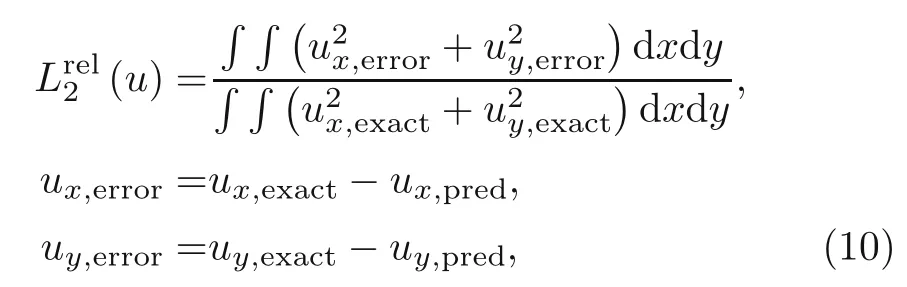
where indices‘exact’and‘pred’indicate the displacements calculated by the exact solution and DEM,respectively.This equation can be found for strain energy as

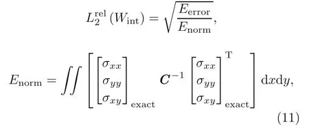
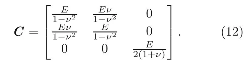
whereEnormandEerrorare the energy norm and energy error,respectively.The stiffness matrix is obtained as follows:

After generating integration points through the Timoshenko beam with the aid of NURBS patches,the energy norm and energy error can be calculated as follows:

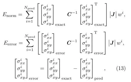
wherewiand|J|are the Gaussian quadrature weights and Jacobean matrix determinant,respectively.

An example of a DEM solution with three hidden layers each containing 30 neurons for a Timoshenko beam with the mechanical and geometrical properties is shown in Table 2.In addition,160 and 40 elements for the longitudinal and vertical axes are considered,respectively,while 80 elements for the boundary domain are considered.The number of Gauss integration points in both boundary and physical domains is 1.The stress distribution of these beams after loading is demonstrated in Fig.6.Consequently,the magnitude of loading at the free end of the beam is 2.

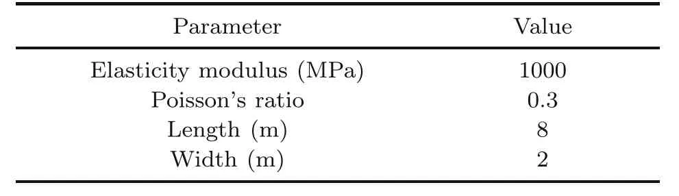
Table 2 Mechanical and geometrical properties of the Timoshenko beam

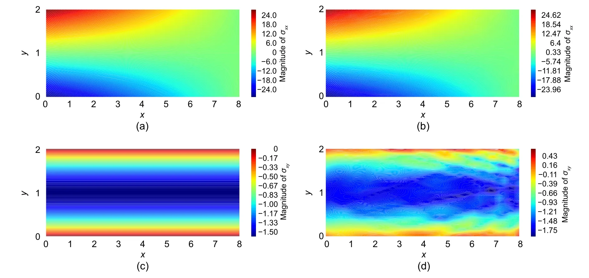
Fig.6 Comparison between the results of analytical solution and DEM:(a) σxx obtained by exact solution;(b) σxx obtained by DEM;(c) σxy obtained by exact solution;(d) σxy obtained by DEM.References to color refer to the online version of this figure

The relativeL2error in the displacement and energy norms for the cantilever beam problem are 0.000 15 and 0.0281,respectively,after 1000 epochs of training.The accuracies of predicting shear and normal stresses are almost the same,although the predicted normal stresses are more in line with the analytical solution compared to shear stresses.Thus,the errors of shear stresses in Fig.6 are more visible because they are depicted relative to the scale of the values of shear stresses(between−1.6 and 0),which is much smaller than the values of normal stresses(between−24 and 24).This can be proven by comparing the mean absolute errors(MAEs)of shear and normal stresses as

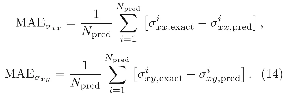
The MAE associated with shear and normal stresses calculated by the DEM solution with network architecture of [30,30,30] are 0.0724 and 0.0588,respectively.These errors are at the same level,and DEM is capable of accurately predicting shear stresses as normal stresses.

4.1.2 Plate with a circular hole in the center

This section considered a square plate with a circular hole in the middle subjected to uniform traction at infinity.Thus,only a quarter of them is studied due to the symmetry of these plates(Fig.7).

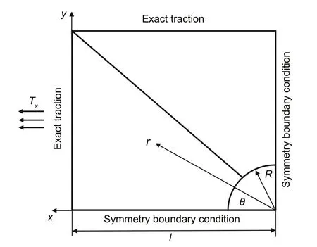
Fig.7 A schematic of a square plate with a circular hole in the middle under uniform traction

According to the study presented by Anitescu et al.(2018),the exact displacements of this plate are calculated as:

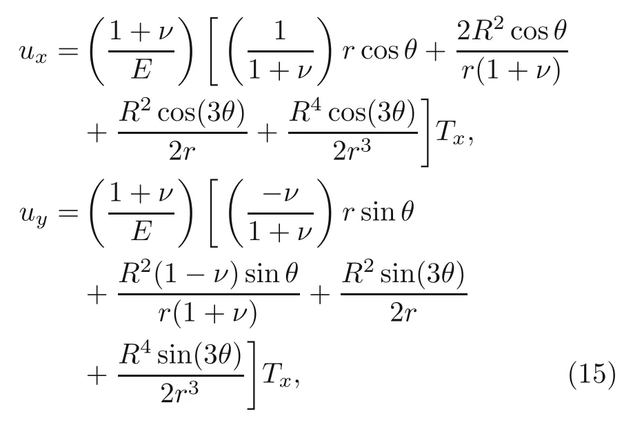
wherer,R,θ,andTxare shown in Fig.7.

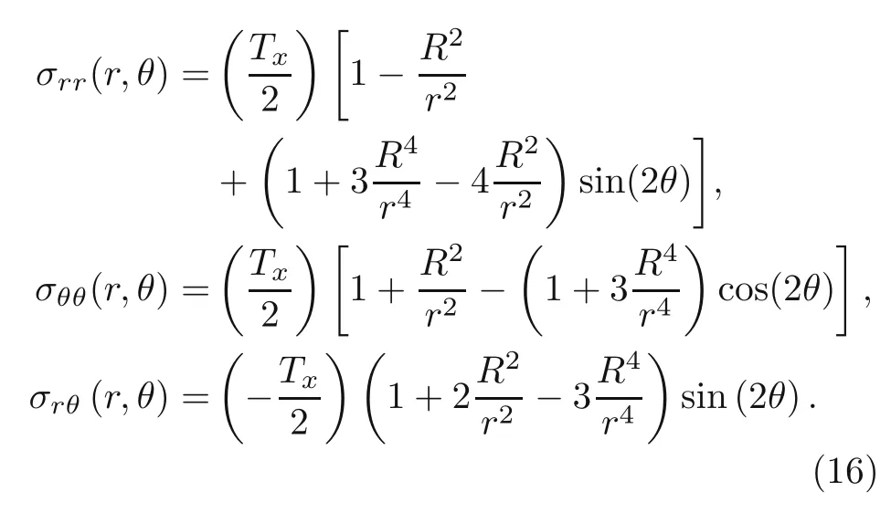
The analytical stress distribution through these plates can be calculated as:

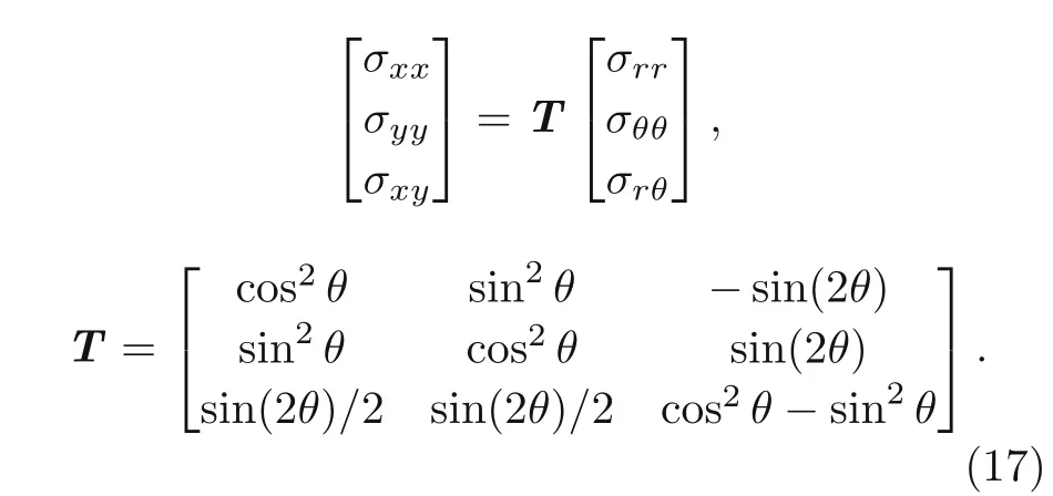
Moreover,the above calculated stresses can be obtained in the Cartesian coordinates using the transformation matrix:

The structure is described by NURBS patches to analyze these plates using DEM.Moreover,a certain number of Gauss integration points are generated in each element to calculate all the integrations after generating elements through the plate.A schematic of the distribution of Gauss points through these plates is depicted in Fig.8.

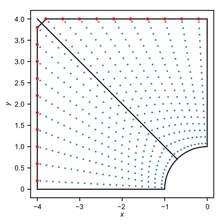
Fig.8 A schematic of the generated integration points through the square plate with a circular hole in the middle.References to color refer to the online version of this figure

The elements are created in the radial and angular directions.The small blue and big red points in Fig.8 represent the Gauss integration points through the body and boundary,respectively.After generating the integration points,a DNN with a specific network architecture is created to be applied on the integration points and predict the relativeL2energy error as the loss function.Subsequently,the network is trained for several iterations until the discrepancy between the analytical method and DEM is minimized.Finally,the displacement and stress distributions of these plates are calculated.The relativeL2errors associated with displacements and energy are calculated similar to the previous section(Eqs.(10)–(13)).

Moreover,Samaniego et al.(2020)implemented DEM to investigate the behavior of a square plate with a length of 4 m containing a circular hole with a diameter of 1 m under uniform traction with a magnitude of 10 MPa.The elasticity modulus and Poisson’s ratio of this plate were 100 GPa and 0.3,respectively.The network structure,activation function,and optimizers are similar to the DEM used for the Timoshenko beam problem.

Moreover,Fig.9 shows the stress distribution of these plates.The relativeL2errors for displacements and energy of this plate compared to the exact solution were 0.0099 and 0.0267 for 4000 epochs of training,respectively.

The shear stress predicted by DEM with predefined network architecture showed noticeable error compared to the exact solution (Fig.9).However,normal stress distribution through the plate was calculated with negligible discrepancies.

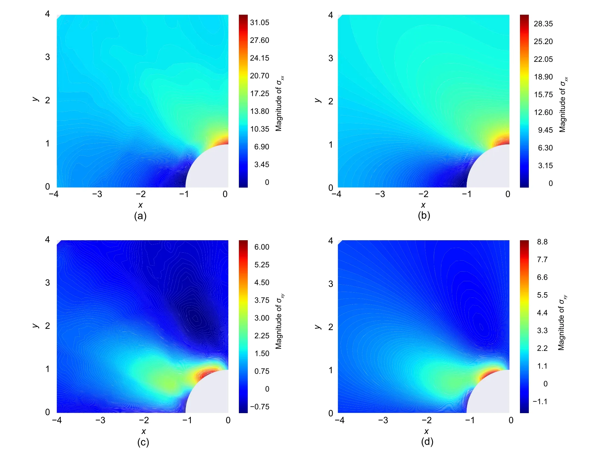
Fig.9 Comparison between the results of analytical solution and DEM with predefined network architecture:(a) σxx obtained by DEM;(b) σxx obtained by exact solution;(c) σxy obtained by DEM;(d) σxy obtained by exact solution.References to color refer to the online version of this figure

4.2 Hyperparameter selection

Various hyperparameters exist (e.g.the number of hidden layers,and the numbers of neurons in each layer,optimizer,and activation function) in a fully connected deep learning problem.However,it is computationally expensive to consider all of them in the process of finding their best set.Therefore,this section used several DEM problems with predefined network architecture to find the results related to various activation functions and optimizers.Finally,the best optimizer and activation function are selected,and the rest of the hyperparameters are optimized in the next section of this study.

4.2.1 Optimizer

This subsection discussed the influence of the optimizer on the prediction accuracy through the backpropagation procedure.Therefore,the results associated with three different optimizers namely root mean square (RMS),Adam,and the combination of Adam optimizer with L-BFGS-B are compared.In the aforementioned optimizer,the network is trained for a certain number of epochs.Subsequently,the training is continued using L-BFGS-B so that the difference between the successive loss functions is <10−8.Moreover,Table 3 shows the comparison between these three optimizers for the cantilever beam with the geometrical and material properties reported in Table 2.The learning rate and the number of training iterations are 0.001 and 1000,respectively.

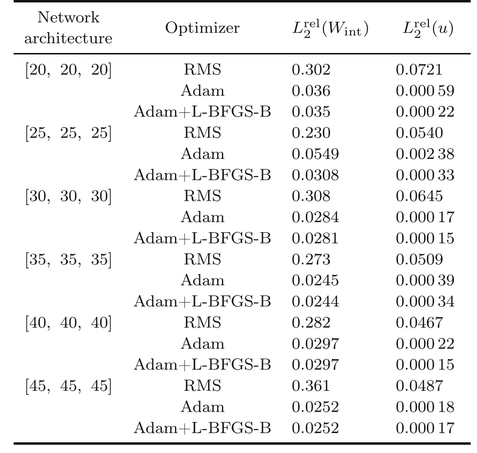
Table 3 Comparison between the results of different optimizers,analyzing the bending of the Timoshenko beam

The comparison of the mentioned optimizers are also presented for the plate with a hole problem in Table 4.The corresponding networks are trained for 4000 epochs and a learning rate of 0.001.

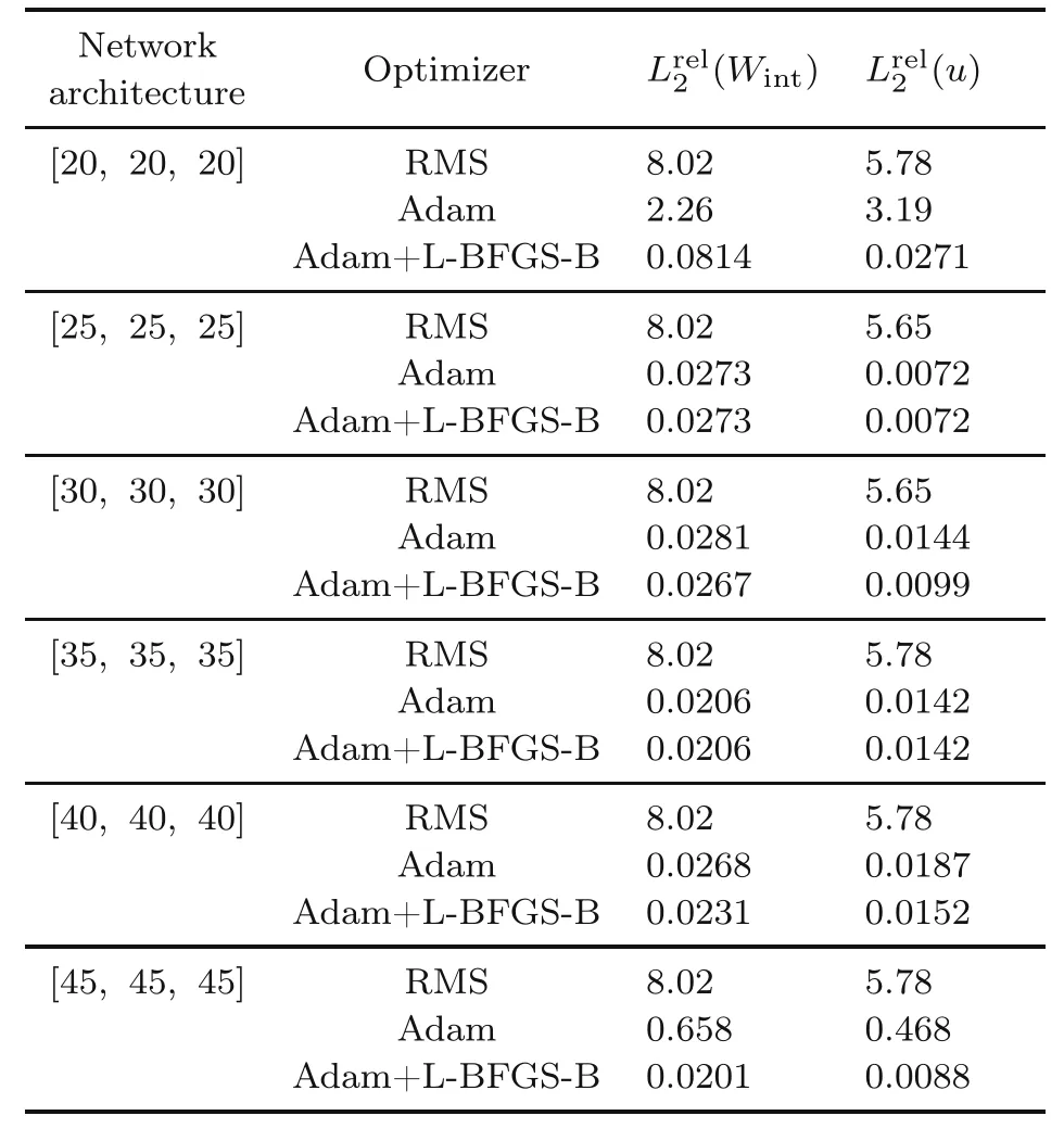
Table 4 Comparison between the results of different optimizers,analyzing the plate with a central hole

Tables 3 and 4 show the huge RMS errors.The Adam optimizer mostly yields accurate results and is outperformed by the combination of Adam and LBFGS-B,particularly when the number of neurons decreases.This is more evident when studying the plate with a hole problem.Thus,the Adam optimizer followed by L-BFGS-B is employed in the rest of this study.

4.2.2 Activation function

Several activation functions,i.e.Sigmoid,tanh,ReLU,and ReLU2,are considered in this study.Moreover,the results are compared in Figs.10 and 11 for the Timoshenko beam and the plate with a hole problem,respectively.

The ReLU is not capable of predicting accurate results for the Timoshenko beam problem(Fig.10),and ReLU2outperforms the other activation functions(Fig.11).Therefore,it was used in this study.

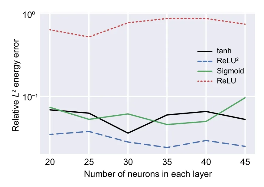
Fig.10 Comparison between the different activation functions in the process of DEM analyzing the Timoshenko beam

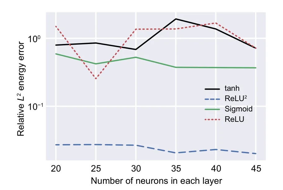
Fig.11 Comparison between the different activation functions in the process of DEM analyzing the plate with a central hole

4.3 Optimization of DEM hyperparameters

4.3.1 Timoshenko beam

The main focus of this study is to exploit GA to find the best DEM hyperparameters.The results of optimizing the DEM network architecture on a Timoshenko beam with material and geometrical properties reported in Table 2 are presented in this subsection.Thus,three NN models with two,three,and four hidden layers are taken into consideration.Moreover,three different sets of integration points,reported in Table 5,are considered to find the influence of the number of integration points on the GA convergence and optimal hyperparameters.

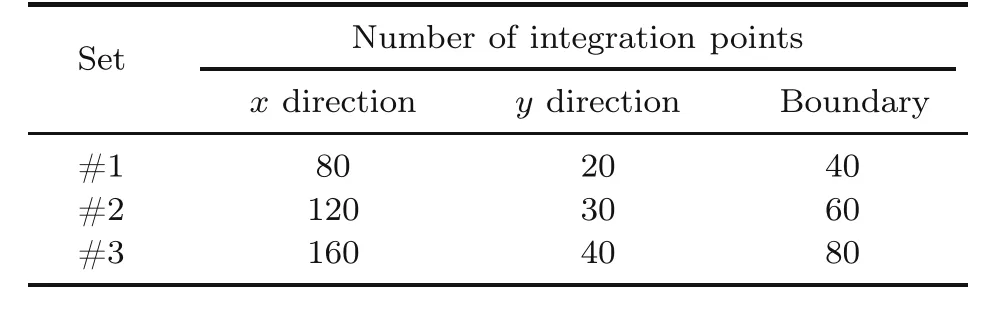
Table 5 Three sets of integration points through the Timoshenko beam

For the sake of simplicity,these sets of integration points are written as {T1,T2,T3} whereT1,T2,andT3are the numbers of integration(training)points in thexdirection,in theydirection,and at the boundary,respectively.For instance,set #1 is noted as{80,20,40}.Moreover,different DEM network architectures are written as[N1,N2,N3]whereN1,N2,andN3are the numbers of neurons in the first,second,and third hidden layers,respectively.

As the process of NN takes a significant amount of time during the GA and quite a large number of NNs during each GA iteration,it is a rational idea to decrease the computational costs by altering the input data of this problem.Therefore,the range of the number of neurons in each layer is lowered,as the number of hidden layers increases,so that the total number of neurons is constrained to a certain maximum.Accordingly,the upper and lower bounds of the neurons in each layer of different GA problems are reported in Table 6.

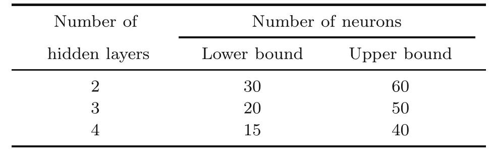
Table 6 Lower and upper bound constraints of the number of neurons for different DEM approaches

The convergence procedures of GA approaches for DEM with two,three,and four hidden layers are demonstrated in Figs.12–14,respectively.

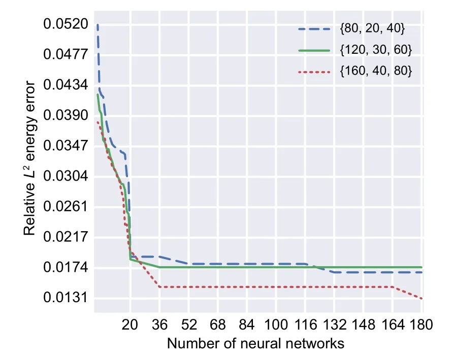
Fig.12 GA convergence applied on the two-layered DEM (Timoshenko beam)

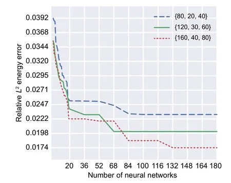
Fig.13 GA convergence applied on the three-layered DEM (Timoshenko beam)

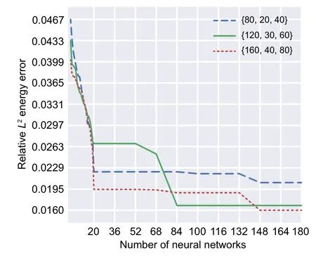
Fig.14 GA convergence applied on the four-layered DEM (Timoshenko beam)

GA successfully decreased the relativeL2error associated with the energy of the Timoshenko beam as the objective function(Figs.12–14).Interestingly,the best results are represented by a two-layered DEM with integration points of {160,40,80}.The corresponding relativeL2error is 0.0131,and the optimum design parameters are 41 and 39 neurons in the first and second layers,respectively.

The four-layered DEM approaches are less accurate compared to their two-layered counterparts.The objective function of GA converges to 0.016 for DEM with integration points of{160,40,80}where the optimum numbers of neurons in layers 1,2,3,and 4 are found to be 30,19,17,and 17,respectively.

The worst optimum results are related to threelayered DEM approaches.The best optimum hyperparameters among the three-layered DEM is related to that with integration points of {160,40,80} and 46,24,and 43 neurons in the first,second,and third hidden layers,respectively.

Another descriptive comparison between the optimal hyperparameters of the different NN models with different numbers of integration points is demonstrated in Fig.15.More detailed results such as energy norm,relativeL2error associated with displacements,and computational time of these approaches are reported in Table 7.

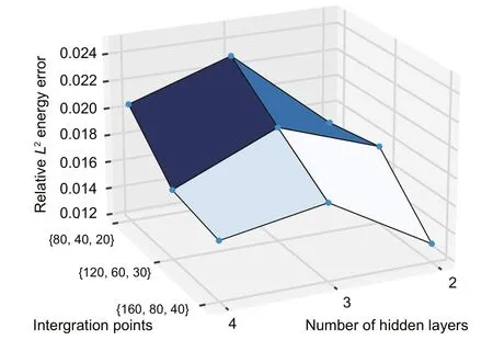
Fig.15 The optimal results of GA on DEM (Timoshenko beam) with various integration points and numbers of hidden layers

Table 7 shows that among all of the optimum results obtained by the GA,the best result is related to DEM with two hidden layers containing 41 and 39 neurons and the integration points of {160,40,80}.In addition,increasing the number of integration points significantly improves the minimized objective function.Furthermore,33%,32%,and 28%decreases in the relativeL2energy error can be seen in the two-,three-,and four-layered DEM approaches,respectively,by increasing the number of integration points to {160,40,80}.To more clearly depict the influence of optimizing the DEM hyperparameters on the stress distribution of the Timoshenko beam,the normal and shear stresses through the analyzed beam are demonstrated for the twolayered DEM with the network architecture of [41,39] and set of integration points of {160,40,80}(Fig.16).

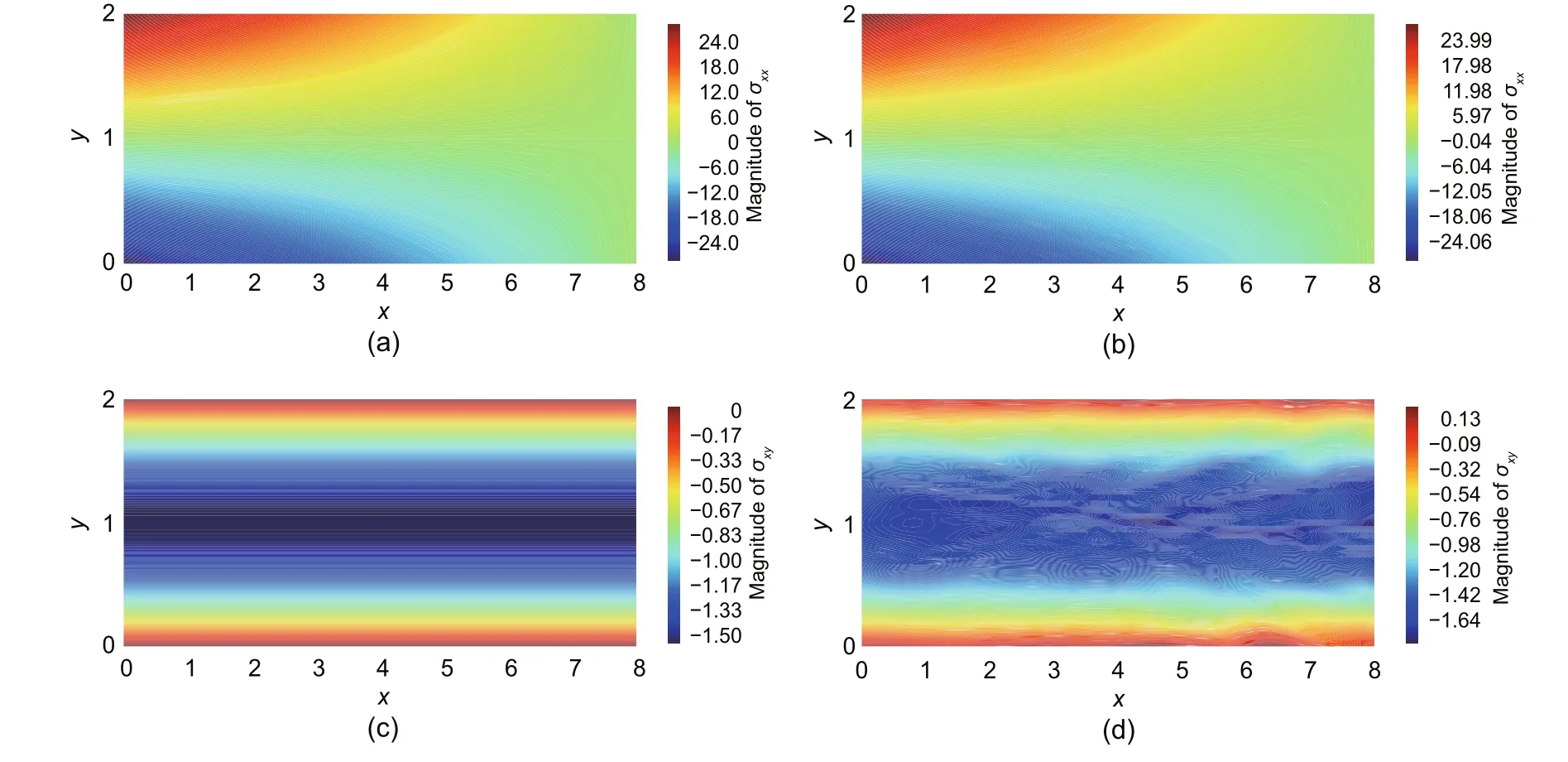
Fig.16 Comparison between the results of the analytical solution and optimized DEM (network:[2,41,39,2]):(a) σxx obtained by exact solution;(b) σxx obtained by the optimized DEM;(c) σxy obtained by the exact solution;(d) σxy obtained by the optimized DEM.References to color refer to the online version of this figure

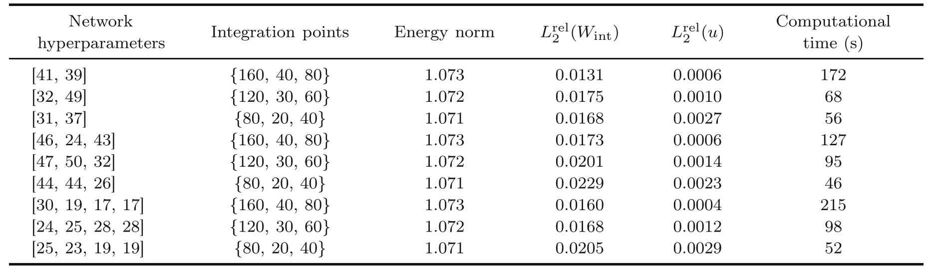
Table 7 Detailed comparison between the optimal results of DEMs on Timoshenko beam with various integration points and numbers of hidden layers

The results related to normal stress for DEM with predefined network architecture are accurate enough as per comparison of Figs.6 and 16.In addition,the accuracy of this stress component does not considerably change by optimizing the network hyperparameters.Consequently,the shear stresses predicted by the optimized DEM are noticeably more accurate than those of DEM with predefined threelayered NN,each containing 30 neurons.Moreover,the MAEs associated with normal and shear stresses,obtained by DEM with a network architecture of[41,39]are 0.0427 and 0.0298,respectively.These errors are 27% and 59% less than the errors produced by DEM with the network architecture of [30,30,30],respectively.Therefore,MAE as another error estimator,shows the significant influence of optimizing the DEM hyperparameters on the accuracy of predicting stress distribution.

4.3.2 Square plate with a circular hole in the center

In this example,the same square plate with a hole studied by Samaniego et al.(2020) is investigated,and the hyperparameters of the NN in the DEM solution are optimized using GA.Thus,a three-layered NN,with each layer containing 20 to 50 neurons,is selected.Furthermore,the numbers of neurons in these layers are considered as the design variables while the relativeL2error associated with energy is taken as the objective function.The GA procedure is presented for three different sets of integration points with 60,70,and 80 integration points in the radial and angular directions as well as the plate boundary.The convergence of the implemented GA is shown in Fig.17.

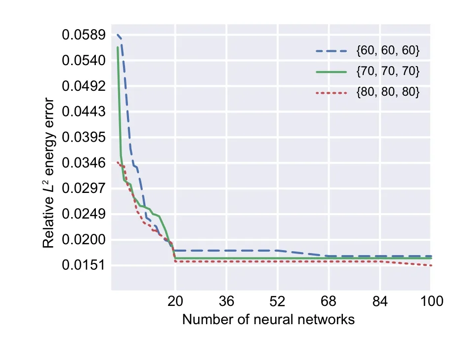
Fig.17 GA convergence applied on the three-layered DEM (square plate with central hole) considering the number of neurons in each layer as the design variable

Optimizing the network architecture (number of neurons in each hidden layer)has a significant influence on DEM accuracy (Fig.17).The optimal network architecture found for the set of integration points {60,60,60} is [39,42,48],which leads to a relativeL2energy error of 0.0169.The DEM accuracy slightly increases by increasing the number of integration points so that the optimal network architecture for the set of integration points {70,70,70}is [35,33,45],which results in a relativeL2energy error of 0.0165.The best optimum network belongs to the set of integration points{80,80,80}with network architecture of [30,41,44],which yields to a relativeL2energy error of 0.0151.However,the objective function decreases 43% when compared with the optimal network architectures with a predefined three-layered network with each layer containing 30 neurons.Detailed results containing energy norm,relativeL2error associated with displacements,and computational time of optimized DEM with different sets of integration points are shown in Table 8.

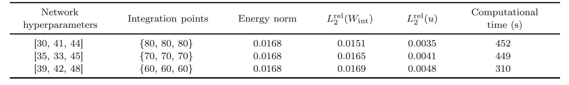
Table 8 A detailed comparison between the optimal network hyperparameters of DEMs on the plate with a central hole for various sets of integration points

The DEM stress distribution with network architecture of[30,41,44]and set of integration points{80,80,80} is depicted in Fig.18 to show the GA influence on the DEM accuracy.

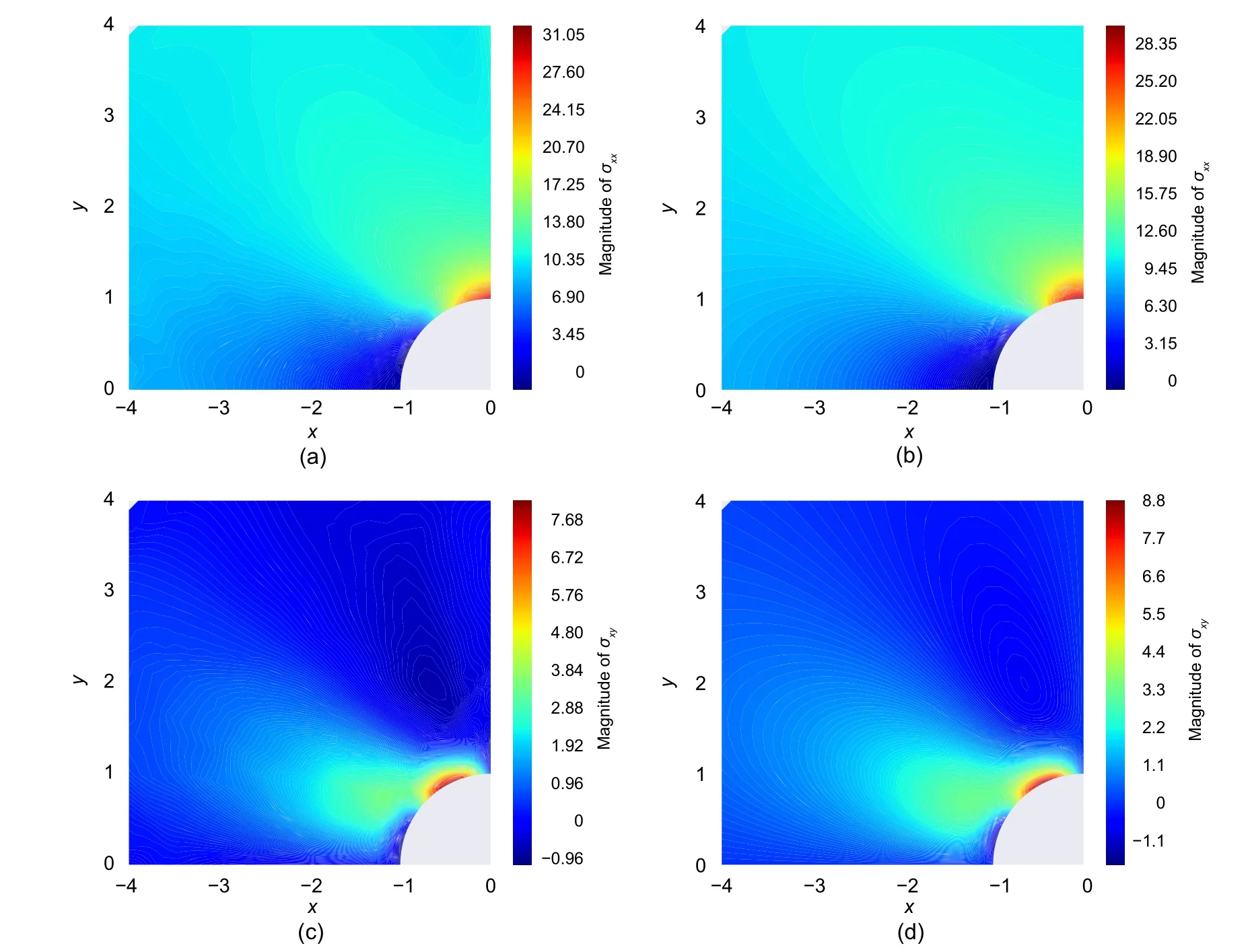
Fig.18 Comparison between the results of analytical solution and DEM (network:[30,41,44]):(a) σxx obtained by DEM;(b) σxx obtained by exact solution;(c) σxy obtained by DEM;(d) σxy obtained by exact solution.References to color refer to the online version of this figure

Optimizing the network architecture has a slightly positive influence on the normal stress of the plate when Figs.9 and 18 are compared.However,the network with optimized architecture [30,41,44]proves to be significantly more powerful than the network with predefined architecture[30,30,30]in terms of predicting shear stresses.

4.3.3 Optimizing the integration points for NN with predefined architecture

In the previous examples,the number of integration points was fixed and the best neural network architecture (the number of neurons in each hidden layer)was found using GA.A certain NN is selected and the optimal combination of integration points is optimized in this section using GA.Thus,the stress analysis of a plate containing a circular hole in the middle with mechanical and geometrical properties reported in the previous example is solved usingDEM.Three NNs consisting of three hidden layers,each containing 30,35,and 40 neurons,are chosen to find the optimal set of integration points for each network architecture.The number of integration points through the structure and the boundary varies from 60 to 90.Moreover,Fig.19 demonstrates the GA convergence in optimizing the number of integration points.

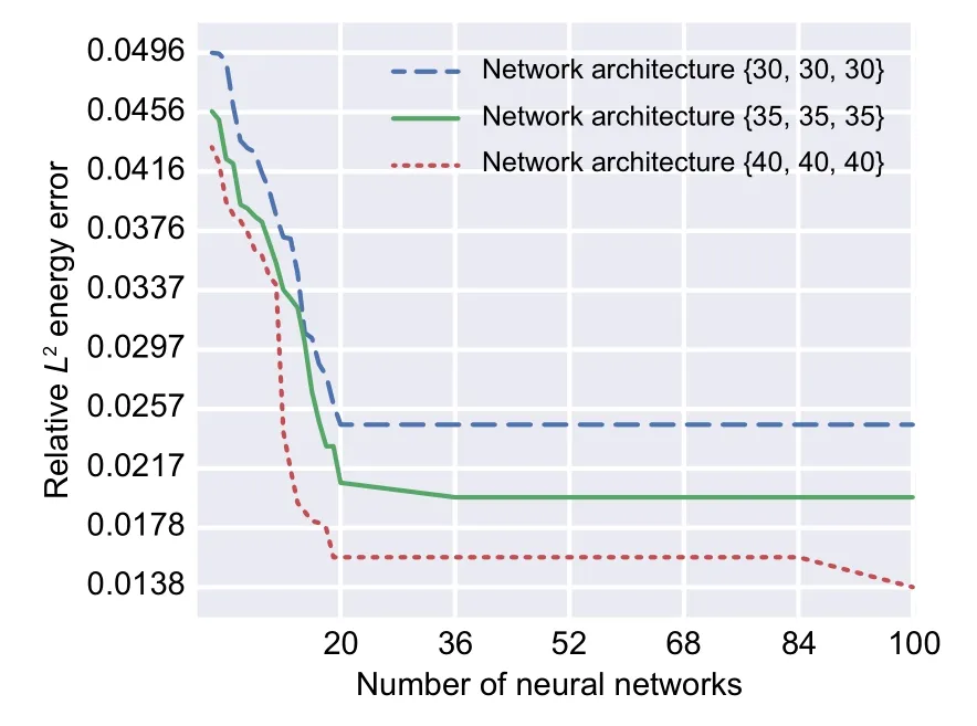
Fig.19 GA convergence applied on the three-layered DEM (square plate with central hole) considering the number of integration points as the design variable

Optimizing the number of integration points when the network architecture is fixed could decrease the loss function up to 50% (from 0.0496 to 0.0247)as shown in Fig.19.Comparing the DEM results with the optimized set of integration points {76,76,70}with the predefined set of integration points{80,80,80},the relativeL2energy error decreased about 8% (from 0.0267 to 0.0247).This clarifies that the predefined set of integration points was properly chosen.This amount could even further decrease up to about 26% (from 0.0267 to 0.0198) and about 48%(from 0.0267 to 0.0138)when increasing the number of neurons in each layer from 30 to 35 and 40,respectively.The detailed report of optimal results related to NNs with the various numbers of neurons in each layer is revealed in Table 9.

4.3.4 Overfitting

The main goal of every supervised ML algorithm is generalization,which is defined as the capability of a trained model to cope with unseen data and to predict the labels of unseen data as accurately as the training data.Two terminologies,overfitting and underfitting,in ML represent the incapability of modeling a set of data.On the one hand,underfitting occurs when the ML approach cannot model training data nor test data.On the other hand,overfitting refers to the ML approach which can predict the labels of training data too well so that they are completely matched with the training data and their accuracy in estimating the labels of test data is poor.

The accuracy of the optimized NN in predicting the stress distribution of the Timoshenko beam was excellent as shown in previous sections.However,investigating whether the adopted models encounter overfitting or not is important.Thus,a new set of integration points is defined as the test data,and DEM solutions with two and four hidden layers are applied to it.Subsequently,the procedures of converging the axial and shear stresses at specific points through the DEM process for the training and test data are compared.Table 10 shows the numbers of integration points of training and test data in thexandydirections.

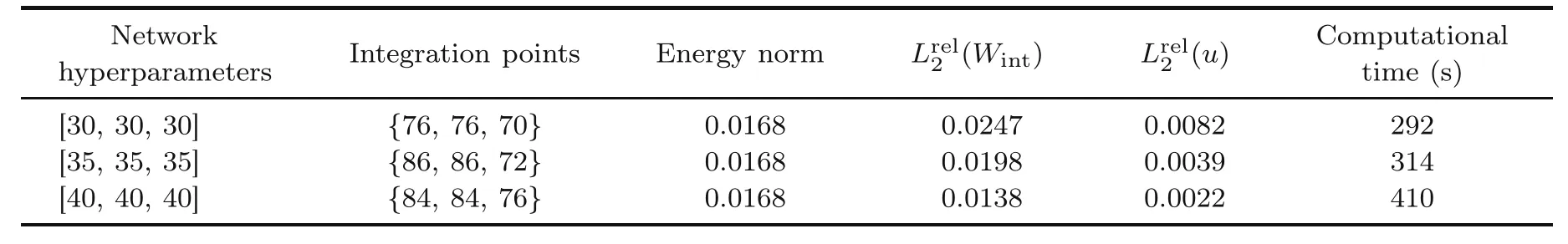
Table 9 A detailed comparison between the sets of optimal integration points of DEMs on the plate with a central hole for various network hyperparameters

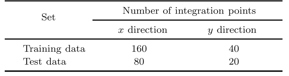
Table 10 Numbers of integration points in training and test datasets

The main sign of overfitting while using NN in solving various problems is that the training dataset converges towards the exact results,whereas the test dataset diverges.As shown in Figs.20 and 21,the training and test data behave in line with each other,and the results associated with normal and shear stresses of these datasets converge to the analytical results as the number of iterations increases.Therefore,the represented DEM solutions with optimized network architecture and sets of integration points do not encounter overfitting and are reliable.

5 Conclusions

GA was used in this study to find the NN optimal hyperparameters in DEM with the relativeL2energy error as the objective function.A cantilever Timoshenko beam with specified geometrical and material properties was chosen as the first case study.Three different numbers of integration points and three different numbers of hidden layers were investigated to find that the best optimal

hyperparameter architecture belonged to the twolayered network with 41 and 39 neurons in the first and second layers,respectively.The numbers of integration points for this optimal network design were 160,40,and 80 in thexdirection,in theydirection,and at the boundary,respectively.The relativeL2energy error of this optimum design was 0.0131,which is a >50% decrease compared to a three-layered DEM approach with 30 neurons in each layer(0.0281).Eight other optimal designs exist for other combinations of the numbers of hidden layers and integration points which resulted in relative energy error between 0.016 and 0.023.

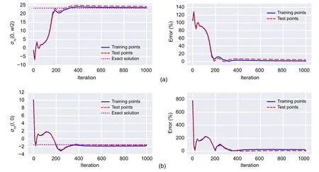
Fig.20 Convergence of stresses through the DEM process with network architecture of [41,39]:(a) normal stress at the top surface of the fixed end;(b) shear stress at the middle of the free end

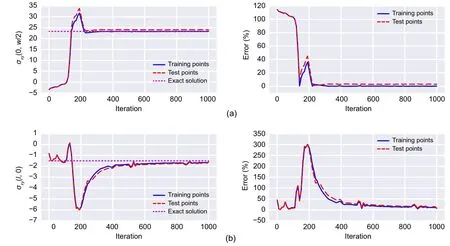
Fig.21 Convergence of stresses through the DEM process with network architecture of [30,19,17,17]:(a)normal stress at the top surface of the fixed end;(b) shear stress at the middle of the free end

The second case study was a square plate with a central hole under traction.The results associated with this structure were also promising.GA introduced the optimal network architecture [30,41,44]yielding to a relativeL2error of 0.0151 (decreasing>38%)compared to the DEM solution with a predefined network[30,30,30]which led to the relativeL2energy error of 0.0247.The set of integration points in both of the mentioned DEM solutions was{80,80,80}.

The network architecture was fixed and the number of integration points was taken as the design variable of the GA process in another example provided in this article.This led to a network architecture of [40,40,40] and a set of integration points of{84,84,76}when analyzing the plate with a central hole.The relativeL2energy error for this optimal design was 0.0138,which is 44% less than the DEM solution with predefined parameters.

The accuracy of predicting the stress distribution through both of the studied structures was also significantly increased by optimizing the NN hyperparameters in DEM.Although a vast number of NNs are conducted in this study to reach the optimal hyperparameters,remarkable improvement in the accuracy of the model would be an acceptable compensation.Combining different approaches in this study and simultaneously conducting an optimization on NNs considering the numbers of integration points,hidden layers,and neurons in each layer as the design variables are highly recommended.

Contributors

Timon RABCZUK devised the project,verified the computational process,and contributed to the final version of the manuscript.Mohammad SALAVATI contributed to the simulation process.Arvin MOJAHEDIN worked out the technical details,performed the computational calculations,and wrote the manuscript.

Conflict of interest

Arvin MOJAHEDIN,Mohammad SALAVATI,and Timon RABCZUK declare that they have no conflict of interest.