Damage detection in steel plates using feed-forward neural network coupled with hybrid particle swarm optimization and gravitational search algorithm*

Long Viet HO，Duong Huong NGUYEN，Guido de ROECK，Thanh BUI-TIEN，Magd Abdel WAHAB

1Soete Laboratory,Department of Electrical Energy,Metals,Mechanical Constructions and Systems,Faculty of Engineering and Architecture,Ghent University,Gent 9000,Belgium

2Department of Bridge and Tunnel Engineering,Faculty of Civil Engineering,University of Transport and Communications,Ho Chi Minh 700000,Vietnam

3Department of Bridge and Tunnel Engineering,Faculty of Bridge and Road,National University of Civil Engineering,Hanoi,Vietnam

4Department of Civil Engineering,Structural Mechanics,Katholieke Universiteit Leuven,B-3001 Leuven,Belgium

5Department of Bridge and Tunnel Engineering,Faculty of Civil Engineering,University of Transport and Communications,Hanoi,Vietnam

6Division of Computational Mechanics,Ton Duc Thang University,Ho Chi Minh City,Vietnam

7Faculty of Civil Engineering,Ton Duc Thang University,Ho Chi Minh City,Vietnam

Abstract:Over recent decades，the artificial neural networks (ANNs) have been applied as an effective approach for detecting damage in construction materials.However，to achieve a superior result of defect identification，they have to overcome some shortcomings，for instance slow convergence or stagnancy in local minima.Therefore，optimization algorithms with a global search ability are used to enhance ANNs，i.e.to increase the rate of convergence and to reach a global minimum.This paper introduces a two-stage approach for failure identification in a steel beam.In the first step，the presence of defects and their positions are identified by modal indices.In the second step，a feedforward neural network，improved by a hybrid particle swarm optimization and gravitational search algorithm，namely FNN-PSOGSA，is used to quantify the severity of damage.Finite element (FE) models of the beam for two damage scenarios are used to certify the accuracy and reliability of the proposed method.For comparison，a traditional ANN is also used to estimate the severity of the damage.The obtained results prove that the proposed approach can be used effectively for damage detection and quantification.

Key words:Feedforward neural network-particle swarm optimization and gravitational search algorithm (FNN-PSOGSA);Modal damage indices;Damage detection;Hybrid algorithm PSOGSA

1 Introduction

One of the most important challenges in structural health monitoring is to identify damage in the considered structures.Damage identification plays a crucial role in the normal operation and maintenance processes of a structure.A vibration-based damage identification method is one among many non-destructive methods，such as those using X-rays or ultrasonic waves.The presence of damage can cause changes in the dynamic properties of structures，e.g.their natural frequencies，displacement mode shapes，and damping ratios.Therefore，many researchers have used these modal properties for damage detection，localization，and severity quantification.It is easy to obtain natural frequencies by using the dynamic response of structures.A simple excitation induced by a hammer blow or under ambient load (Ho et al.，2019;Nguyen et al.，2020a) can provide values of natural frequency，and mode shapes of laboratory beams with high accuracy.Ho et al.(2020) used piezoelectric sensors to obtain the vibration frequencies of cables of a real cable-stayed bridge under ambient load.These are the most popular parameters used for damage assessment.However，environmental conditions，including temperature，have significant effects on the changes of natural frequencies.On the Z-24 bridge in Switzerland，after one-year of monitoring，a variation from 14% to 18% in the first four frequencies due to environmental changes was revealed by Peeters and de Roeck (2001).These effects can cause miscalculation of damage in structures.Mode shapes are more stable with temperature variation than are natural frequencies (Xia et al.，2006;Moser and Moaveni，2011).Hence，displacement mode shapes are also used for damage assessment.However，for higher modes，it is not easy to acquire smooth mode shapes.A method using the second derivative of mode shapes was investigated by Pandey et al.(1991) who proposed a new damage detection method，termed the modal curvature method (MCM).This approach delivered promising results for defect identification when using a large number of points in the measurement grid.A modal flexibility method was also proposed by Pandey and Biswas (1994) for failure detection and localization.A modal flexibility index contains both frequencies and mode shapes.From their studies，they confirmed that the estimation of the flexibility matrices was easier and more accurate，even with a few lower modes.This makes this method attractive because these lower modes are easier to measure.Pandey and Biswas (1995) successfully verified their proposed method using experimental data.Other researchers also investigated the efficiency of the modal flexibility method for the detection and localization of damage.Wickramasinghe et al.(2015) applied the modal flexibility method to the numerical vibration properties of suspended cables to localize the damage.From the obtained results，the lateral vibration modes were most important for damage detection and localization.Dawari and Vesmawala (2013) generated numerical data of damage in concrete beams.They applied modal flexibility and modal curvature methods for defect identification.From the observed results，they indicated the successful application of the two methods for honeycomb damage detection.Accuracy and simplicity of computation and application are the main advantages of the modal flexibility method.Therefore，this technique is widely used in damage identification.However，damage quantification based on these modal damage indices remains a challenge for the engineering community.

To solve this problem，many researchers took advantage of optimization algorithms to determine the location as well as the extent of damage.Tran and Bui (2019) were successful in using particle swarm optimization (PSO) for damage detection in a steam beam based on experimental results.Zhu et al.(2017) suggested a hybrid objective function，consisting of frequency and coordinate modal assurance criterion (COMAC) for damage identification.Results of defect identification have proved that this approach is promising due to its high accuracy and simplicity.However，the shortcoming of this approach is its time-consumption.The technique needs to re-run for many damage scenarios in order to analyse and predict the failure for each input dataset.For this reason，the learning ability of artificial neural networks (ANNs) performs much better.Through learning from a sufficient training dataset，the trained networks make their own diagnosis when unlearned data are input.In other words，the training process is conducted once，but the trained network can be used for different input datasets.This means that the computational time is significantly reduced.

Applications of ANNs in engineering problems are very diverse.The bending behaviour of a Kirchhoff plate was analysed using a deep collocation method.The approach is based on a feedforward deep neural network and has the advantages of computational graphs and backpropagation algorithms.The proposed method was used for plates with boundary conditions，as well as numerous shapes (Guo et al.，2019).Another solution to solve partial differential equations (PDEs) was suggested by Anitescu et al.(2019).In this approach，ANNs and an adaptive collocation strategy were used to solve the boundary values problem.The obtained results showed good accuracy.An energy approach to the solution of PDEs was presented by Samaniego et al.(2020).In this study，deep neural networks based on the deep energy method and the collocation method were considered as a function approximation of a PDE.The capabilities of the proposed approach were evaluated through applications in computational mechanics.Recently，many researchers successfully used the learning ability of ANNs to quantify damage levels.Nguyen et al.(2020b) were successful in proposing a novel approach to determine multiple cracks in a beam under a moving load.This method is a combination of wavelet analysis and deep learning.Firstly，based on the static displacement signal，wavelet analysis can point out the location and quantity of damage.Then deep learning uses dynamic elements to evaluate the growth rate of damage.Tran-Ngoc et al.(2019) combined a cuckoo search algorithm and ANN for defect localization and quantification in a bridge and a beam-like structure，using frequencies as input of the neural network.A damage index was developed by Garcia-Perez et al.(2013) for defect localization using a combination of wavelets and empirical mode decomposition.The results showed good potential in applications to damage location identification in truss-like structures.Nguyen et al.(2019) coupled transmissibility and ANN for damage detection.Numerical data of a bridge under moving loads were used to investigate the effectiveness of the proposed approach.However，the first and simplest type of ANN，the so-called feedforward neural network (FNN)，is the subject of this paper.In FNNs，the inputs are passed on hidden layers by a transfer function to achieve outputs of hidden layers.Then the hidden layers continue to pass on output layers to obtain the final outputs.In other words，the information is forwarded from input nodes，through hidden nodes to output nodes in this network.However，random sets of biases and weights do not always result in a good fit between estimated and desired values，and errors can be significant.A common way to improve the estimated results is to use a backpropagation neural network.In this procedure，these learning errors are used to adjust the values of biases as well as weights.Then，these biases and weights are input again in the network to obtain final outputs until a stopping criterion is met (Fig.1).This means that these errors are used to refine the proposed neural network to improve the predicted outputs.In supervised learning，a backpropagation neural network is a common training algorithm for FNNs.However，the gradient-based algorithm suffers from stagnation in local minima instead of the global minimum and slow convergence.

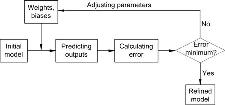
Fig.1 Overview of back propagation neural network

In general，the aim of the learning process is to achieve values of biases and link weights that can minimize the error between the target and predicted values.Recently，many heuristic optimization algorithms have proved their ability in local minima avoidance，fast convergence，and high accuracy.Using the advantages and diversity of optimization algorithms opens up high applicability to solve particular problems thoroughly.For instance，Le-Duc et al.(2020) developed balancing composite motions (BCMO) for solving varieties of the optimization problems.No algorithm-specific parameter was needed in creating the algorithm.The robustness and effectiveness of the proposed optimization algorithm were confirmed through applications in three real engineering design problems.For this reason，some researchers used heuristic optimization algorithms for FNN training to solve benchmark problems such as the iris/breast cancer classification problem and function approximate problem.Zhang et al.(2007) used backpropagation combined with PSO.Valian et al.(2011) applied an improved cuckoo search algorithm.With the aim of reducing the potential of being trapped in local minima and increasing the convergence rates，Mirjalili et al.(2012) used a hybrid PSO and gravitational search algorithm (PSOGSA) for training FNNs，namely FNN-PSOGSA，in iris classification，function approximation，and exclusive or (XOR) problems.Khatir et al.(2017) successfully used a modal flexibility index for delamination identification in composite beam-like structures.Liu et al.(2014) studied the potential application of the neural network and the modal flexibility indicator in damage identification of a beam.However，only four damage severities were collected as training data.

Based on these ideas，we used FNN-PSOGSA and modal flexibility indices to solve engineering problems.In this approach，cuts are simulated in the finite element (FE) model，representing real failures in practice instead of an assumption of reduction stiffness.Many more scenarios of damage levels than in previous studies were used to train neural networks.This guarantees the accuracy and reliability of the proposed approach.

In this study，a simple two-stage method for failure determination was implemented using a numerical simulation of a free-free steel beam.In the first step，modal damage indices，namely modal flexibility indices，are used to identify the location of a defect.In the second step，defect severity is quantified by FNNs improved by PSOGSA.The advantage of this approach is the remarkable reduction in computational time involved in collecting data for training.Because the damaged element is predetermined，only data on the severity of damage at the identified element or in smaller areas are gathered instead of from all elements in the structure.This can improve the accuracy of the approach by reducing the amount of irrelevant data.The inputs of this model are variations of modal damage indices associated with reduction of stiffness，and the outputs are the severities of damage in the structure.

2 Modal flexibility

In general，flexibility has an inverse relationship with the stiffness of structures.The presence of a defect in a structure will reduce the stiffness，leading to an increase in flexibility.Therefore，the modal flexibility index，based on the quantity of shift in flexibility，is used to determine the presence of a failure.

Anp×p-dimensional modal flexibility matrixFof a structure withpdegrees of freedom and number of considered modesq，can be identified by inversing the square of frequencies as

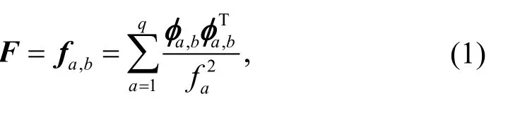
wherefa,bis a component of the modal flexibility matrix，φa,bis a mode shape vector that is normalized to the mass matrix at locationbof modea，andfais the natural frequency of modea.From Eq.(1)，the increase in frequencies can lead to a rapid decrease in the flexibility matrix，and vice versa.Therefore，some first lower modes can be used to achieve a good estimation of the flexibility matrix of a structure.This is the practical meaning of the modal flexibility index.

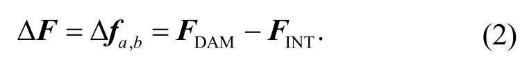
From modal properties consisting of mass normalized mode shapes as well as natural frequencies of intact and damaged states，two flexibility matrices are determined asFINTandFDAM，respectively.Anp×p-symmetric flexibility change matrix △Fis achieved by

A maximum absolute valueδbof elements △fa,bin thebth row (or column) of the flexibility change matrix is given by

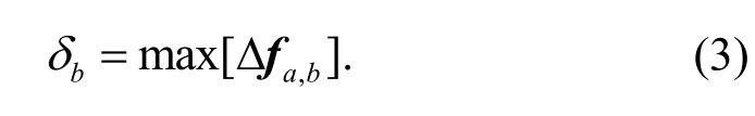
This index then can be used to localize the damage in structures.

3 Feedforward neural network improved by hybrid particle swarm optimization-gravitational search algorithm (PSOGSA)

3.1 PSOGSA

Inspired by PSO and GSA，the hybrid PSOGSA was developed by Mirjalili et al.(2014).It is a combination of the local search capability of GSA and social thinking of PSO.Their studies showed that the best fitness of the objective function was computed faster than using either PSO or GSA，and with a similar accuracy.The superior performance of PSOGSA can be explained by the hybrid algorithm overcoming drawbacks in explorations of PSO and GSA.In PSO，only the personal best of each particlePbestand the global best of all particlesGbestare used to influence each search agent in updating the position at each iteration.In contrast，PSOGSA has the intrinsic feature of GSA:each agent is affected by all agents.This allows PSOGSA to perform better than PSO.In GSA，exploitation in final iterations is slower than that in PSOGSA.When a promising solution is found，search agents gather around the solution for exploitation.In the final iterations，the similar weights of masses lead to the same intensity of gravitational forces.Approximate attraction of these forces to each other slows down the exploitation.PSOGSA inherits social components from PSO，and can exploit neighbouring the best agent obtained.Therefore，in PSOGSA，exploitation is accelerated.

In this algorithm，with two agents having random positionssx，syand Euclidean distances between them，Dxy，and a small constantε，the gravitational forces are calculated as

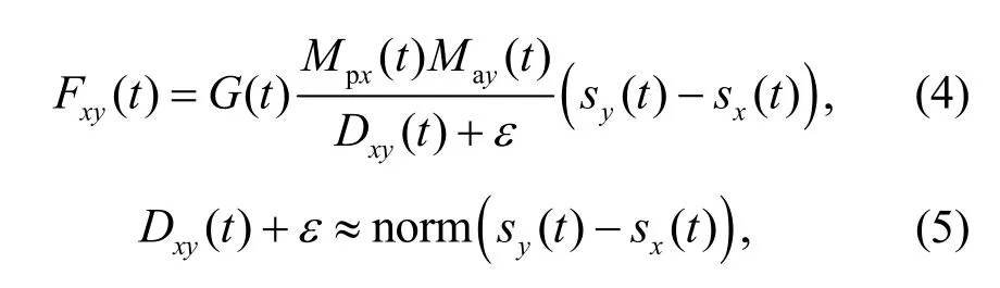
whereG(t) is a gravitational constant，andMpxandMayare the passive and active gravitational masses ofxandyagents，respectively.These parameters can be computed by

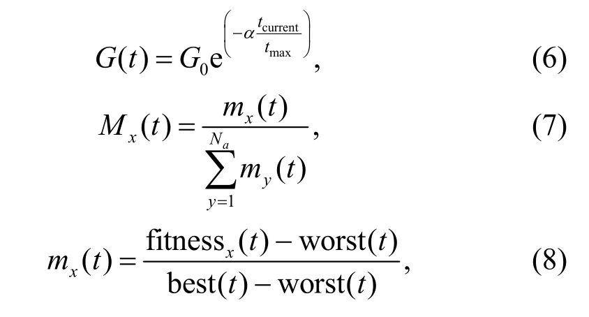
whereG0is the initial value of gravitational constant，αis the reducing coefficient，and best(t)，worst(t)，fitnessx(t) are the best，worst，and current values of fitness，respectively.tcurrentandtmaximply the current iteration and maximum numbers of iterations，respectively.mxandmyare gravitational masses ofxth andyth agents，respectively.

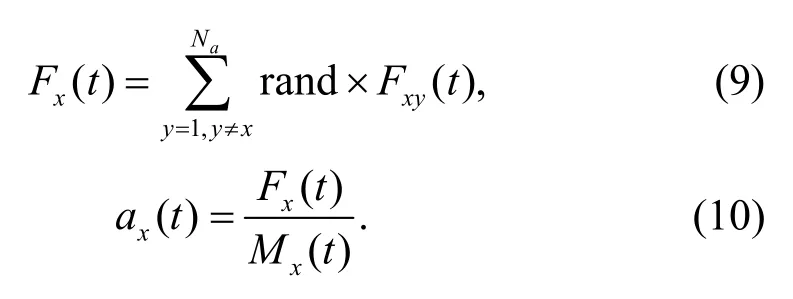
Then，a total forceFx(t) on agentxdue toNanumber of agents is determined by Eq.(9).After that，this obtained force is combined with the mass of agentsMxto generate acceleration of agentxat iterationt，ax(t)，asgiven in Eq.(10).

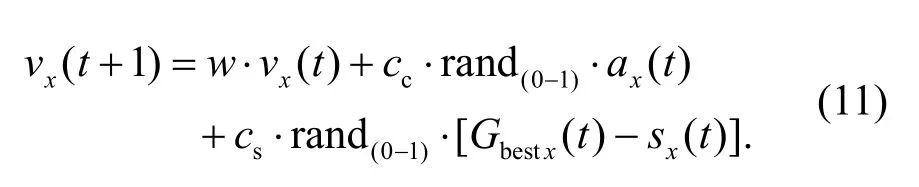
In the next step，the velocities of the agentsvx(t) are updated using the cognitive coefficientccand the social coefficientcsof PSO:

Then，the positions of agents are identified after each iteration:

Stopping criteria，e.g.limiting the maximum iteration or the deviation of values between two successive runs of the fitness function，should be preset.When the termination condition is met，the loop will stop.Details of the GSA and PSO can be found in (Kennedy and Eberhart，1995;Rashedi et al.，2009).

3.2 Training feedforward neural networks (FNNs) using PSOGSA

To overcome the drawbacks of FNNs mentioned in Section 1，this paper focuses on how to train FNNs using a heuristic optimization algorithm.A hybrid algorithm PSOGSA is used to achieve the best set of biases and weights that can effectively reduce the error of FNNs.This means that the error of the FNNs will be used as a fitness function of the suggested method，FNN-PSOGSA.

In this paper，an FNN that includes one input layer，one hidden layer，and one output layer with the structure 2-S-1 is used as plotted in Fig.2，whereSrepresents number of neurons in the hidden layer.The activation function is a sigmoid function.

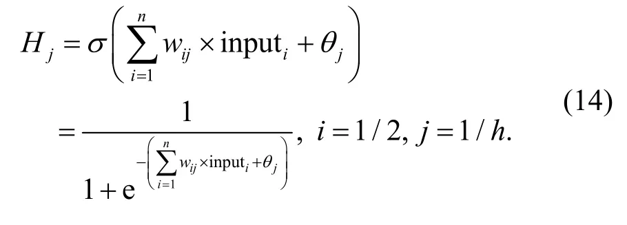
From Fig.2，the numbers of input，hidden，and output nodes are denoted byn，h，andm，respectively.The input of neurons of the hidden layer is calculated as，where inputiis theith input，θjis the bias of thejth hidden node，andwijis the link weight between theith input node andjth hidden node.The sigma symbol in Fig.2 denotes the weighted sum of the previous layer.Then the output of the hidden layerHjcan be calculated as

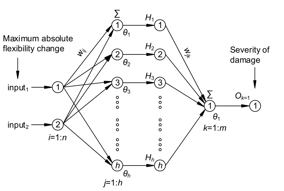
Fig.2 Structure of the proposed FNNs with a 2-S-1 structure (n=2,h=S,m=1)

Final outputs of output layerOkare determined from:

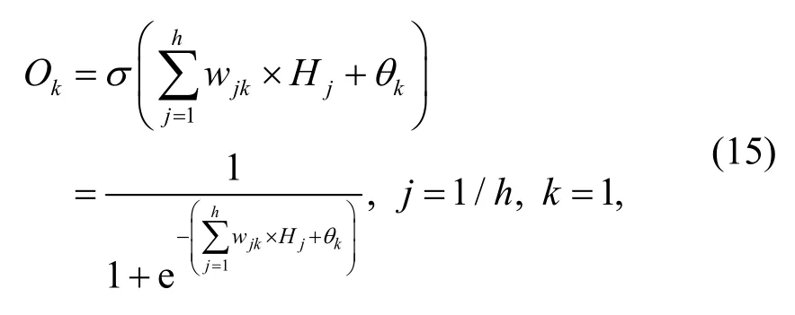
whereθkis the bias of thekth output node，andwjkis the link weight between thejth hidden node andkth output node.

After calculation of final outputs from the output layers，the fitness function used in this study is the learning error，identified as the mean squared error (MSE) based on the sum squared error (SSE):

whereOk(c)andTk(c)are the actual output and target output of thekth output using thecth training sample，respectively，andNSis the total number of training data.

In the data-preparation step，to avoid a very flat transfer function that can lead to a saturated neural network，the training data should be arranged in a suitable range.In this paper，sigmoid is the activation function，therefore the inputs，initial weights，and outputs should be chosen in a range of from 0.01 to 0.99 or −1.0 to 1.0 based on specific problems (Rashid，2016).The procedure for using PSOGSA for training FNNs is shown in Fig.3.

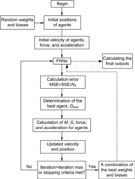
Fig.3 Flowchart of FNNs improved by PSOGSA

4 Finite element model

In this paper，a free-free beam with a rectangular cross-section is modelled by ANSYS 17.0.The natural vibration of the beam without effects of supports was the major reason for choosing a free-free beam.In the FE model，a 1-m-beam was constructed using 16 elements.The 6th element was used to generate damage scenarios.For damaged as well as healthy states of the beam，modal properties，e.g.frequencies and displacement mode shapes，are collected for damage detection and quantification.

Two scenarios of damage at the same location are considered (Fig.4).The first includes a left cut and the second consists of a left cut and a right cut.

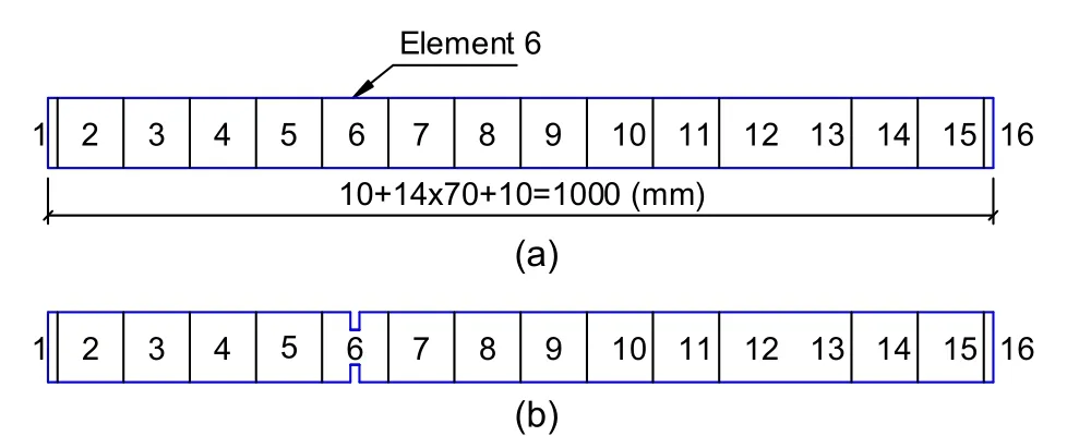
Fig.4 Intact (a) and damaged (b) free-free beams

4.1 Input parameters

The material properties of the steel are:Young’s modulusE=2.0×1011N/m2，density=7820 kg/m3，and Poisson’s ratiov=0.3.Dimensions of the rectangular cross-section of the beam areb×h=71.356 mm× 9.817 mm.The total length of the beamL=1000 mm.The cuts are:5.000 mm-width，and the length of cuts，bcutvaries from 1% to 20% of the total width of the beamb.For further tests，two cuts were considered withbcut=12.5 mm for the left side andbcut=12.3 mm for the right side.This generated two damage levelsbcut/b=17.24% and 34.76%.The location of the cuts is 325 mm from the end of the beam.Details of the two cuts are plotted in Fig.5.

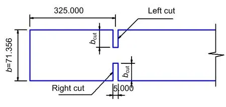
Fig.5 A damage scenario of the beam (unit:mm)

Solid element 185 in ANSYS was used to construct free-free FE models of a steel beam.These models included one intact and two damage states (Fig.6).A convergence study was conducted for a solid model and four elements were generated through the thickness of beam.

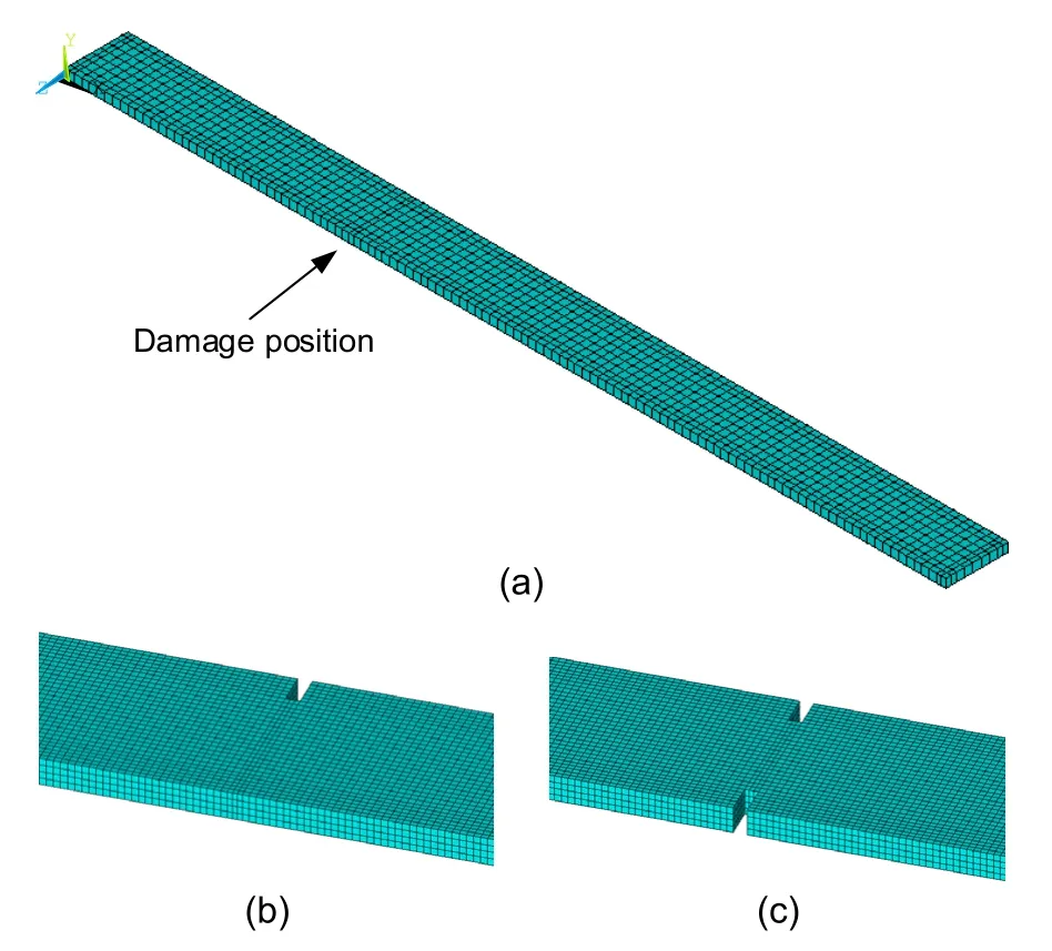
Fig.6 FE models using solid 185 and details of cuts:(a) FE model in 3D-view;(b) one cut;(c) two cuts

In (Nguyen et al.，2020a)，types of elements，e.g.beam element，shell element，and solid element，were used to investigate the variation of mesh size of the FE model.The converged frequencies obtained from the FE model showed a good agreement with the experimental frequencies.All errors in frequencies between the FE model using solid elements and measurements were under 1%.Therefore，the same elements and mesh size were used to build the FE model in this study.This guaranteed good accuracy of the FE results.Details of the convergence study are given by Nguyen et al.(2020a).

4.2 FE results

Modal analysis was conducted using ANSYS 17.0.The first five vertical bending modes of intact and damage states are shown in Fig.7.

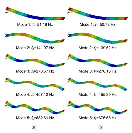
Fig.7 Five calculated mode shapes:(a) intact beam;(b) damaged beam with two cuts

5 Damage localization and quantification

5.1 Damage localization using modal flexibility index

The FE models of the intact and damaged beams were constructed to obtain frequencies and displacement mode shapes.The aim of the study was to localize a random position of damage.Therefore，a random position in Fig.5 was generated.Another goal of the study was to investigate the capability of the proposed approach in response to a shift in severity.An extra cut at the same location represents an increase in the extent of damage.Using real cuts is more practical than assuming a stiffness reduction.Many previous studies modelled stiffness reduction by reducing Young’s modulus.In this study，the FE model can consider the decrease of stiffness as well as the loss of mass.Then，the modal flexibility matrices are calculated using Eq.(1).Data of the displacement mode shapes are collected from the nodes shown in Fig.8.Then，damage locations are identified using the maximum absolute values of the flexibility change matrix using Eq.(3).Some damage scenarios at 5%，15%，25%，and 35% were investigated to determine the modal flexibility indices using the first mode，the first three modes，and the first five modes.Damage localization results of the modal flexibility indicator are shown in Figs.9 and 10.

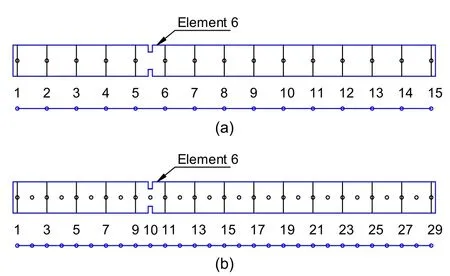
Fig.8 Schematic diagram of nodes used to collect displacement mode shapes

In the first case，from the obtained results，the change in the modal flexibility indices reveals the damaged region in an interval from node 9 to node 11 (two vertical black dash-dotted lines) when the first mode，the first three modes or all the first five modes are used.Fig.9b and Fig.9c indicate the damage location at point 10 more exactly and clearly than in Fig.9a.In other words，the clear peaks in Figs.9b and 9c accurately pinpoint the position of the defect.This also shows the promising performance when just the first few lower modes are used.

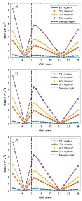
Fig.9 Flexibility change for four scenarios of damage severity for the free-free beam using one mode (a),three modes (b),and five modes (c) of 29-node model

In the second case，the grid points are reduced to verify the feasibility of method for real applications where a limitation of sensors is of significant concern.In this case，displacement mode shapes of 15 nodes，as mentioned above，are collected.Similar to the first case，the defect localization shows superior results when more mode shapes are used.Although the index cannot show the exact location of the damage，it delineates the failure zone between nodes 5 and 6 (Fig.10).This confirms that this method is very useful to determine the location of failure with the first few modes and a proper number of sensors.

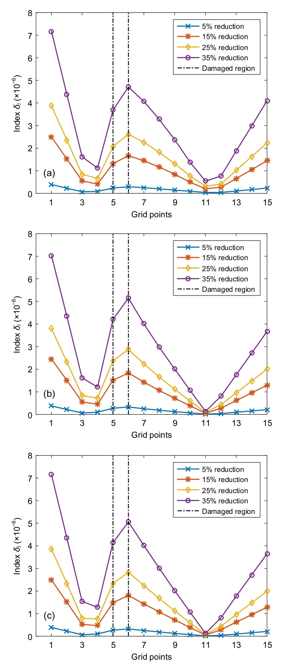
Fig.10 Flexibility change for four scenarios of damage severity for the free-free beam using one mode (a),three modes (b),and five modes (c) of 15-node model

The damage location has already been determined in this section.Therefore，the maximum absolute flexibility change indicesδiat two nodes 5 and 6 in the second case are gathered for damage quantification in the next section.This contributes to reducing the computational time and increasing the accuracy of severity level estimation.

5.2 Damage quantification using FNN-PSOGSA

In this step，40 scenarios of damage severities from 1% to 40% are generated with two cuts in the beam，for training.Based on the obtained modal properties of healthy and damaged structures，the maximum absolute flexibility changeδiis calculated.

By means of the training procedure，the values of weightwijand biasesbjof FNNs are updated.These values then are re-input into the neural network to quantify the failure level.Two extra damage scenarios at 17.24% and 34.76% are generated and used to verify the reliability and accuracy of the suggested approach.Natural frequencies of the intact and damaged beams are shown in Table 1.

Some pre-set parameters for PSOGSA based on the study of Mirjalili et al.(2012) are:the number of agents 30，the gravitational constantG0=1，and the cognitive coefficientccand the social coefficientcslying in [0，2].In this case the cognitive coefficientcc=1，the social coefficientcs=1，α=20，initial inertia weight reduces linearly fromwmax=0.9 towmin=0.4 asw=wmax−tcurrent×(wmax−wmin)/tmax，and random values in a range of 0 to 1.0 are assigned to the initial velocities of agents (particles).

For FNNs，inputs，connection weights，and desired outputs (targets) are normalized in a range of from 0.01 to 0.99 due to its better convergence than in the range of from −1.0 to 1.0 after a test run.An FNN with the structure 2-S-1 is used to identify the level of damage.The performance with the numbers of hidden nodes，S=5，15，25，and 35 is investigated with the numbers of independent iterationsN=500 andN=1000.Table 2 shows the best MSE for all training data.Fig.11 shows the convergence curves based on the MSE of FNN-PSOGSA over 500 and 1000 iterations.Random training samples are used during the training process instead of consistent samples.

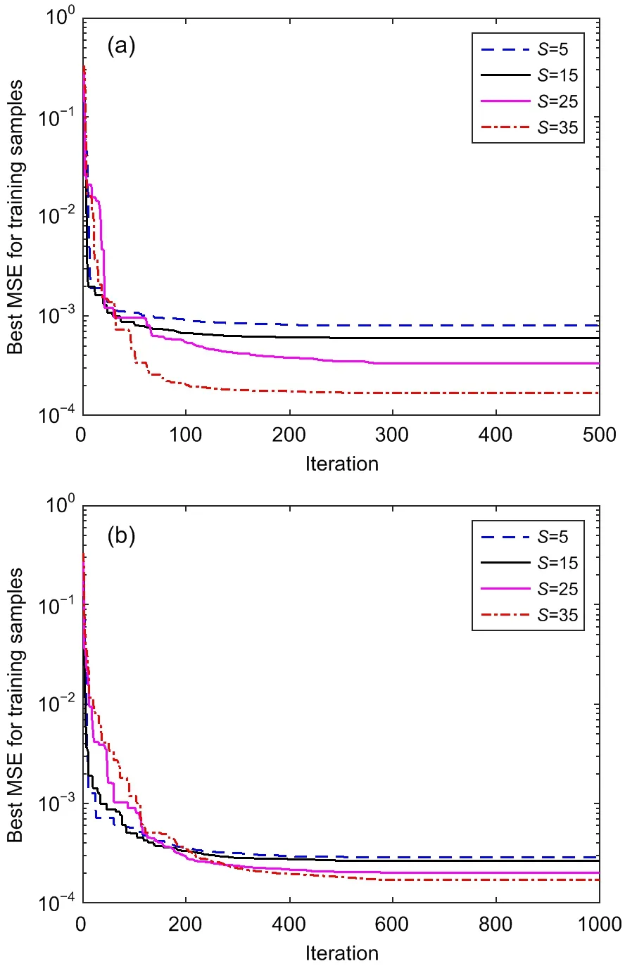
Fig.11 Convergence curves of FNN-PSOGSA associated with number of hidden nodes S=5,15,25,35:(a) 500 iterations;(b) 1000 iterations

The obtained results reveal that the number of hidden nodes，S=35，achieved a superior result with the best MSE.This is reasonable because the larger the number of hidden nodes，the slower the convergence，and the smaller the learning error.Figs.11a and 11b make this point very clear.

To guarantee the accuracy of prediction using FNN-PSOGSA，some hyper-parameters such as the initial population，the cognitive coefficientcc，and the social coefficientcswere investigated in two cases.In the first case，the numbers of the population are 20，30，40，50，and 60 with two coefficientscc=cs=1.In the second case，based on the optimised population in the first case，the variation of two coefficientsccandcsin a range of [0.5，2] is studied.In each case，one investigated parameter is run 20 times.The training process is stopped when the maximum number of iterations，Itermax=1000.

Values of the average MSE，best MSE，and the standard deviation of MSE (Std MSE) are used to identify the best values of the hyper-parameters.Tables 3 and 4 show that population=50，cc=1，andcs=1 performed better than the others for the standarddeviation of the MSE and the average MSE.The convergence curves in Fig.12 also reveal that the obtained values are suitable for the next step，i.e.damage identification.

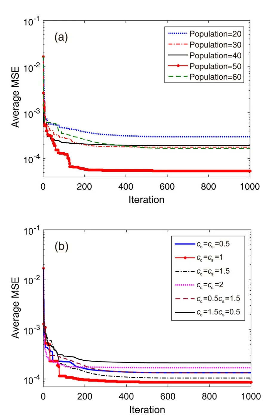
Fig.12 Convergence curves using FNN-PSOGSA based on the average MSE:(a) case 1,variation of population with cc=cs=1;(b) case 2,variation of cc and cs with population=50

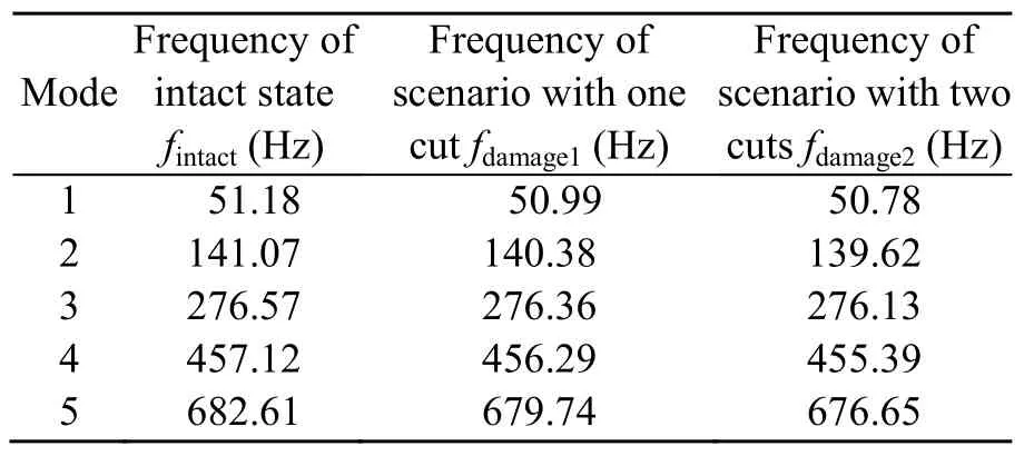
Table 1 Frequencies of the intact beam and damaged beam with two cuts at 17.24% and 34.76%

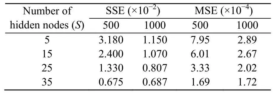
Table 2 The best SSE and the best MSE of FNN-PSOGSA over 500 and 1000 iterations

Therefore，damage quantification of the beam uses FNNs with a structure of 2-35-1 over 10 000 independent runs.Initial hyper-parameters of the population=50，cc=1，andcs=1 are used for PSOGSA.

The best MSE values are plotted against the number of iterations in Fig.13.It can be seen that the convergence curve almost levels off from 6000 iterations onward.Results of predicting the severity of damage are shown in Table 5.

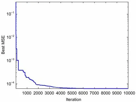
Fig.13 Convergence curves of FNN-PSOGSA with number of hidden nodes S=35 over 10 000 iterations

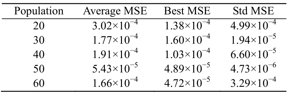
Table 3 The standard deviation of MSE,best MSE,and average MSE over 20 runs associated with different populations

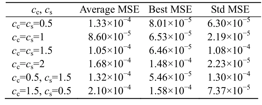
Table 4 The standard deviation of MSE,best MSE,and average MSE over 20 runs associated with different cc and cs

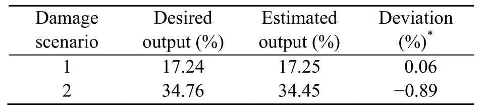
Table 5 Results of damage quantification using FNN-PSOGSAs

The errors between the real (desired) and estimated damage levels are negligible:0.06% and −0.89% for the first and second damage scenarios，respectively.This shows that the proposed method works successfully for damage quantification.

The neural network tool in MATLAB is used to estimate damage levels based on given damage data with the same structure 2-35-1 (Fig.14).In this figure，wandbare the connection weight and bias，respectively.To achieve a superior prediction from ANNs，a network training process needs to be implemented.There are many catalogues of training functions，like quasi-Newton algorithms，conjugate gradient，and gradient descent.A comparative study of training algorithms used to train neural networks was conducted by Sharma and Venugopalan (2014).They revealed two outstanding training functions for neural network training，namely Levenberg-Marquardt (trainlm) and scaled conjugate gradient (traingscg).Du and Stephanus (2018) made a similar assessment of the effectiveness of Levenberd-Marquardt based on their research.For this reason，the Levenberg-Marquardt algorithm was used as a training algorithm in this study.For a good classification of ANNs，the dataset is split into two sets，one for training，and another for validation and testing.A common proportion，70%–30%，was chosen in this study based on the idea that more training data give more accurate error estimation.The splitting dataset (40 samples) includes 70% (28 samples) for training the model，15% (6 samples) for validation，and 15% (6 samples) for testing.

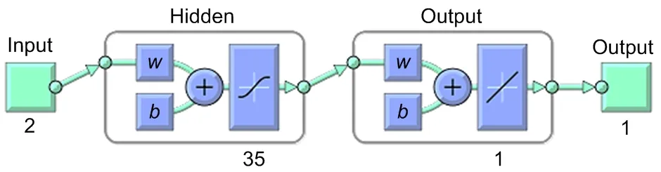
Fig.14 Neural network architecture

Fig.15 shows the regression diagrams of the network outputs concerned with targets for training，validation，and test sets.Almost all data located along a 45° line andRvalues in training，validation，and testing，are over 0.99.We can conclude that the fit is extremely good for all datasets.

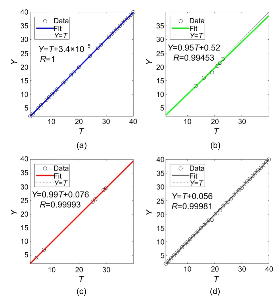
Fig.15 Regression diagrams for training (a),validation (b),and testing (c),and all data (d)

Based on the biases and weights obtained from the neural network，results of identification of damage levels are shown in Table 6.

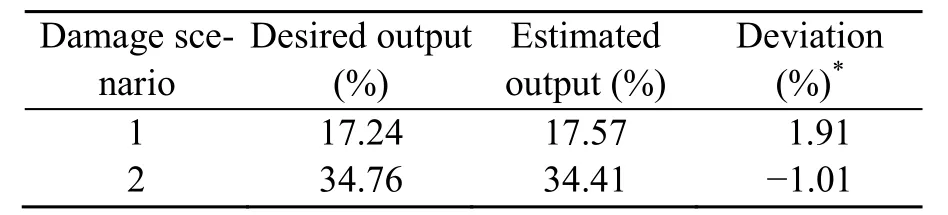
Table 6 Results of damage quantification using traditional artificial neural network (ANN)

A slight difference between the real and estimated damage level is obtained using ANN:1.91% and −1.01% for the two damage cases.Fig.16 shows a visual comparison between FNN-PSOGSA and ANN.Clearly，the predicted severity using FNN-PSOGSA is better than that of ANN for both damage scenarios.

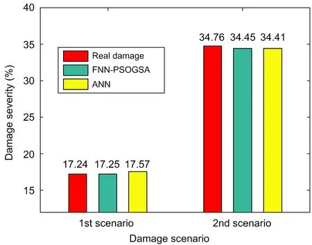
Fig.16 Comparison of damage severities estimated by FNN-PSOGSA and ANN

6 Conclusions

This paper focused on how to implement a heuristic optimization algorithm for achieving the best set of biases and connection weights for an FNN for an engineering problem.The content of the method is based mainly on the global search of the optimization algorithm PSOGSA instead of the backpropagation procedure of traditional ANNs.The negligible discrepancies of defect identification prove that FNN is significantly better than ANN.The superiority of our proposed method is clearly demonstrated by the estimated error of only 0.06% for the first damage scenario versus 1.91% when using ANN.

This study also confirmed the effectiveness of the modal flexibility method in practical application of damage detection and localization.Although only the first three to five modes were used in this study，the maximum absolute flexibility change indices still detected and localized exactly the location of damage as well as the damage zone related to more and fewer measurement points，respectively.

The accuracy of damage quantification using FNN-PSOGSA also proves the feasibility and simplicity of the proposed approach to serve as a potential assessment tool for real structures.

Further study is needed to consider the noise in the measurements，spacing of sensors，and multiple-damage，and to apply the suggested method to a laboratory beam.Validation of the method with experimental data is completely feasible.In the next step，the mass of sensors and the boundary conditions of the tested beam need to be considered carefully.A model updating process has to be carried out to ensure that the intact FE model performs in a similar way as a real one.Then modal flexibility change indices along the beam will be collected both for predicting damage localization and quantification using FNN-PSOGSA.

Contributors

Long Viet HO:methodology，wrote the original draft of the manuscript，software;Duong Huong NGUYEN:helped to organize the manuscript，software;Thanh BUI-TIEN，Magd Abdel WAHAB，and Guido de ROECK:supervision and validation.

Conflict of interest

Long Viet HO，Duong Huong NGUYEN，Guido de ROECK，Thanh BUI-TIEN，and Magd Abdel WAHAB declare that they have no conflict of interest.