Evaluating rock mass disturbance within open-pit excavations using seismic methods:A case study from the Hinkley Point C nuclear power station

Antony Buthr,Ann L.Stork,Jms P.Vron,J-Mihl Knll,b,Ktrin Plnkrs,Finly Booth,Mrus Bonhm,Arin Ko

a School of Earth Sciences,University of Bristol,Wills Memorial Building,Queen’s Road,Bristol,BS8 1RJ,UK

b Department of Earth Sciences,University of Oxford,South Parks Road,Oxford,OX1 3AN,UK

c Gesellschaft für Materialprüfung und Geophysik (GMuG),Bad Nauheim,61231,Germany

d Mott MacDonald,10 Temple Back,Bristol,BS1 6FL,UK

e Atkins,The Hub,500 Park Avenue,Aztec West,Bristol,BS32 4RZ,UK

f Atkins,The Axis,10 Holliday Street,Birmingham,B1 1TF,UK

Keywords:Rock mass strength Rock disturbance Seismic tomography Piezoelectric surveys Picoseismicity Acoustic emissions

ABSTRACT Understanding rock strength is essential when undertaking major excavation projects,as accurate assessments ensure both safe and cost-effective engineered slopes.Balancing the cost-safety trade-off becomes more imperative during the construction of critical infrastructure such as nuclear power stations,where key components are built within relatively deep excavations.Designing these engineered slopes is reliant on rock strength models,which are generally parameterised using estimates of rock properties (e.g.unconfined compressive strength,rock disturbance) measured prior to the commencement of works.However,the physical process of excavation weakens the remaining rock mass.Therefore,the model also requires an adjustment for the anticipated rock disturbance.In practice,this parameter is difficult to quantify and as a result it is often poorly constrained.This can have a significant impact on the final design and cost of excavation.We present results from passive and active seismic surveys,which image the extent and degree of disturbance within recently excavated slopes at the construction site of Hinkley Point C nuclear power station.Results from active seismic surveys indicate that the disturbance is primarily confined to 0.5 m from the excavated face.In conjunction,passive monitoring is used to detected seismic events corresponding to fracturing on the cm-scale and event locations are in agreement with 0.5 m of disturbance into the rock face.This suggests rock disturbance at this site is relatively low and occurred during and immediately after the excavation.A ratio of seismic velocities recorded before and after excavations are used to determine the disturbance parameter required for the Hoek-Brown rock failure criterion,and we assess that rock disturbance is low with the magnitude of the disturbance diminishing more quickly than expected into the excavated slope.Seismic methods provide a low-cost and quick method to assess excavation related rock mass disturbance,which can lead to cost reductions in large excavation projects.

1.Introduction

Quantifying rock strength,and the impact of excavationinduced damage,is essential when undertaking major infrastructure projects.Accurate assessments are necessary for safe and costeffective engineered slopes.Slope stability is a top priority during the construction of critical infrastructure such as nuclear power stations,where key components are built in relatively deep excavations.Determining stress conditions at which a slope will fail,and the amount of rock engineering required to prevent failure,is therefore integral in the design.

The design of these engineered slopes is reliant on rock strength models,which are generally parameterised using estimates of rock properties(e.g.unconfined compressive strength(UCS))measured prior to the commencement of works.However,the physical process of excavation weakens the remaining rock mass through the opening and creation of fractures leading to a reduction in rock strength.Compensating for this disturbance is a crucial component of slope stability assessments.As this disturbance occurs within the rock mass,its severity and extent into the slope are difficult to quantify and often poorly constrained.The resulting uncertainty has a significant impact on the final excavation design,which typically will be over-engineered to ensure an appropriate margin of safety.Here we show how seismic monitoring can provide a nonintrusive method to assess rock damage due to excavation.

The pre-eminent model used for assessing rock mass strength is the Hoek-Brown failure criterion,which was originally developed for underground excavations in hard rock(Hoek and Brown,1980).Following its adoption by the geotechnical industry,it became broadly recognised that,when applied to excavated slopes,the calculated rock mass strengths are overestimated.Consequently,Hoek et al.(2002) presented a major re-examination of the entire Hoek-Brown criterion,which included a new disturbance parameter D,which corrects for a reduction in rock strength caused by excavation damage and stress release.For the majority of rock engineering projects,the level and extent of disturbance are based on visual inspection following Hoek et al.(2002).This qualitative approach is reliant on engineering judgement,informed by reviewing excavation methods and the in situ stress regime.

The volume of the rock mass damaged or altered by mechanical excavation and subsequent stress release due to material unloading is often referred to as the disturbance or excavation damaged zone(EDZ).Rock disturbance causes the creation,dilation and movement of discontinuities,cracks or fractures in a rock mass(Cai et al.,2004)and the large number of factors that influence the degree of disturbance make it difficult to precisely quantity the factor D.Hoek et al.(2002)proposed a set of guidelines based on their experience and published back-analyses of damaged rock,however,these are subjective and contain little detail as to how the values were estimated.In this paper,we use non-destructive geophysical methods to directly measure the extent and degree of disturbance caused by excavation,using a combination of active seismic surveys and passive seismic monitoring.We demonstrate this approach on slopes created during the construction of the Hinkley Point C(HPC)nuclear power station in the southwest of England.

1.1.Excavation effects and rock mass strength

Rock disturbance is described as a reduction in rock mass strength associated with the creation of new discontinuities(cracks and fractures),and dilation/movement of existing discontinuities.Within newly excavated rock slopes,this disturbance is caused by the process of excavation and subsequent stress release.The degree of excavation damage is affected by several factors,including the near-field stress history,rock type,excavation method,and confining pressure (Read,2004),with the process of fracture creation and stress release relatively transient in nature (Lu et al.,2012).

The Hoek-Brown criterion (Hoek and Brown,2019) has been widely adopted within the geotechnical community.This method was employed to assess slope stability at HPC.Unlike the linear Mohr-Coulomb failure criterion,Hoek-Brown criterion follows a nonlinear parabolic form which empirically relates the geological conditions to the rock mass strength based on triaxial test data.Originally developed for the design of underground excavations in hard rock (Hoek and Brown,1980),the criterion has undergone several revisions to make it applicable to general geotechnical applications.This has resulted in the introduction of new parameters,namely rock disturbance (D) and the geological strength index(GSI),which extend the criterion’s applicability to weak rock masses.The generalised Hoek-Brown criterion is expressed by

where σ1and σ3are the major and minor principal stresses,respectively;σciis the UCS of the intact rock material;and mb,s,and a are the constants estimated using GSI,D and the initial material constant,mi,by

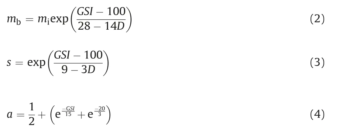
Although the constants have no fundamental relationship with any physical characteristics of the rock,the parameter mbcan be considered analogous to the frictional strength of the rock,and s is related to the rock mass cohesion (Eberhardt,2012).Furthermore,Hoek et al.(2002) proposed the rock mass strength (relation which describes the overall behaviour of a rock mass by

While values of GSI and mican be relatively well constrained through visual assessment of the rock type and extent of jointing(Sonmez and Ulusay,1999),estimating rock disturbance (D) is a more difficult task as it occurs within the rock mass.The degree of disturbance is incorporated into the failure criterion using the parameter D,which ranges between 0 and 1.Where minimal damage occurs to the surrounding rock (e.g.carefully controlled tunnel excavations),then D=0;and if very significant disturbance is induced by activities such as heavy production blasting,then D=1 (Hoek and Brown,2019).The choice of D is critical in the assessment of slope stability,and rock stability can be significantly over-or under-estimated if an incorrect value of D is applied (Li et al.,2011).

Along with an appropriate value of D,the spatial extent of damage into the excavated slope (T) and the time duration over which the disturbance accumulates (i.e.the duration of stress release) are also important parameters in slope design (Fig.1).Currently,common industry practice is to qualitatively assess disturbance through visual inspection of the excavated slope and relate these observations to guidelines published in Hoek et al.(2002).While this provides assessment of the visible slope face,it is unable to determine the extent,variability,and duration of the disturbance within the rock volume.Instead,this analysis often relies on a back-analysis of slope failures to determine both the GSI and D (Sonmez and Ulusay,1999).In this study,we seek to overcome these limitations through geophysical monitoring and surveying during excavations at HPC,with the aim of imaging physical changes in the rock mass.

1.2.Geophysical assessments of rock disturbance

Geophysical methods are rarely employed to assess rock disturbance in slopes similar to those excavated at HPC.Such methods have however been successfully applied in assessments of EDZs resulting from tunnelling or underground excavations (e.g.Martino and Chandler,2004;Cai and Kaiser,2005;Manthei and Plenkers,2018).These studies commonly apply seismic methods that either use active sources to image velocity changes due to the presence of discontinuities(Leucci and De Giorgi,2006;Malmgren et al.,2007;Brodic et al.,2017),or monitor acoustic emissions(AEs)(also called picoseismicity) generated from the formation and movement of cracks and fractures (Cai and Kaiser,2005;Kwiatek et al.,2011;Wang et al.,2019).The two approaches provide complimentary information,with active methods directly measuring seismic P-or S-wave velocities (Vpor Vs) which can be used to constrain the numbers (or fracture density) of newly generated fractures recorded by passive methods.In laboratory settings,Nihei and Cook (1992) combined both approaches to study the seismic behaviour of fractures in sandstone,observing both variations in seismic velocity and AEs with changing confining pressures.In general,these studies focus on rock masses under much higher confining pressures (>20 MPa) than that encountered in the rock slopes at HPC (typically<<1 MPa),but their results demonstrated the capability of seismic methods to assess rock disturbance.

Fracturing in a rock mass strongly affects seismic wave propagation,producing a reduction in transmission velocities,frequency content (Baird et al.,2013;Butcher et al.,2020),and signal amplitudes(Boadu and Long,1996).Seismic velocities can be considered as a bulk measurement of the rock volume,with their sensitivity to fracturing dependent on the frequency of the signal relative to the dimensions of the fractures (Al-Harrasi et al.,2011;Baird et al.,2013).Several relations have been proposed that empirically relate Vpto UCS (Chang et al.,2006;Sharma and Singh,2008;Sarkar et al.,2012)and the rock quality designation(RQD)(Barton,2006;Nourani et al.,2017).RQD is a measure of the percentage of“good”rock recovered from an interval of a borehole (Deere and Deere,1988) and allows for a simple estimation of rock quality which partially relates to the degree of fracturing.McDowell(1993)demonstrated that the ratio of Vpin the field to that measured in the laboratory is numerically equivalent to the RQD,with the laboratory measurement relating to the intact unfractured rock while the field measurement corresponds to the degree of jointing(Barton,2006;Nourani et al.,2017).There are few methods that relate Vpto the Hoek-Brown parameters GSI and D,however,a similar approach used to estimate RQD could be applied to estimating D,since this is also directly related to the degree of fracturing.

Fig.1.Schematic to illustrate rock disturbance parameters resulting from excavation of a rock slope.Within the undisturbed rock,D=0,while within the disturbed rock,D is variable with the largest value encountered at the slope face.

Fig.2.Velocity-pressure model,relating a change in seismic velocity with confining pressure for porous,fractured (solid line),and non-porous (dashed line) rock masses(adopted from Ji et al.,2007).A dilation/opening of pores and fractures sharply reduces velocities (grey area) which is described by the relaxation term,B,with a closing pressure (Pc) occurring when B=0.

While mechanical excavation causes the creation and movement of fractures,stress release causes the dilation or opening of pre-existing fractures and pore space.This release of stress produces an exponential reduction in seismic velocities with confining pressure (Verdon et al.,2008;Asef and Najibi,2013),with several studies empirically relating Vpto the effective pressure (P) at high confining pressures(e.g.Eberhart-Phillips et al.,1989;Ji et al.,2007;Sun et al.,2012).Laboratory measurements of Vpat confining pressures comparable to excavated slopes typically use unconsolidated sediments instead of rock samples (e.g.Prasad et al.,2005),but the same exponential decrease in Vpwith confining pressure was observed due to an increase in pore space and an increase in compliance between grain boundaries.

Vpand P can be related by the model proposed by Ji et al.(2007):

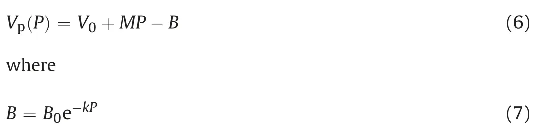
where Vp（P）is the seismic velocity of a porous,fractured medium as illustrated in Fig.2.The model describes the intrinsic properties of a fracture free solid matrix by the parameters V0and M;V0corresponds to the projected velocity without porosity at P=0,while M relates to the elastic volume contraction under pressure.The relaxation term,B,accounts for a dilation of pore space and fractures caused by a reduction in effective pressure,with B0representing the velocity difference between the porous and nonporous materials at P=0.The decay constant,k,controls the shape of the nonlinear segment of the Vp-P curve,which relates to the opening and weakening of compliant pores and fractures.

In the model of Ji et al.(2007),the pressure at which the relaxation term,B,approaches zero is described as the value at which the rock sample is comparable to a fracture-free rock mass.This is referred to the closing pressure (Pc).However,in the lower pressure regime of the shallow subsurface,Pcis instead representative of the pre-excavation confining pressure,when fracture networks,and therefore seismic velocities,are comparable to their pre-disturbance state.Imaging seismic velocity variations,and their return to pre-excavation values therefore provide a useful assessment of the severity and extent of damage within the rock mass.

While the opening of fractures results in a reduction of seismic velocities,their sudden movement can cause a rapid release of energy and the generation of transient pulses of elastic wave energy.These seismic events are produced by shear rock movement as well as tensile opening and compaction.For the fracture size of interest in this study,this produces high frequency(kHz range),low amplitude picoseismic,or AE events (Brune,1970;Bohnhoff et al.,2009),which provide additional information on the condition of the rock mass.As these events relate to slip on fractures,their distribution within the rock mass can be used to complement observed variations in seismic velocities with respect to the degree of fracturing within a rock mass.Nihei and Cook (1992) observed this relationship within a laboratory setting where an exponential increase in velocity with pressure was observed but only a more gradual increase in AEs with pressure was observed,with fewer events occurring at lower confining pressures.This suggests that monitoring picoseismicity may be best suited for determining the maximum extent of fracturing within the rock mass.

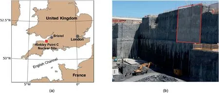
Fig.3.(a) Location of Hinkley Point C,and (b) image of excavated slope used in this study.The red box indicates the area in which geophysical surveys were undertaken.

2.Hinkley Point C (HPC) and ground excavations

HPC,located in the southwest of England(see Fig.3),is the first in a new generation of nuclear power stations to be built in the UK.It will be comprised of two nuclear reactors (Units 1 and 2),and when operational in mid-2020s,it will generate approximately 6%of the UK’s electricity.The earthworks involved in the construction are significant;excavations extend up to 35 m below ground level and in total approximately 5.6 million m3of earth will be moved.The deepest excavations are located within the region of the heat sink,where 2 km long intake tunnels will draw water from the Severn Estuary to cool the power station.

Within the heat sink excavations,we monitored a 10 m wide section of the slope during excavation to a depth of 15 m below ground level.This monitoring area was considered representative of the geological setting,and the findings from this study were used to optimise the future design of the remaining excavation.The objective was to provide revised estimates of rock strength that are calibrated using geophysical measurements.

The bedrock geology at HPC consists of mudstones,shales,and limestones of the Blue Lias,Lilstock,and Westbury formations,which overlay the mudstone beds of the Blue Anchor and Red Mudstone formations(Green,1992).The majority of the excavated slope in this study is within the Angulata and Upper Liasicus Biozone of the Blue Lias formation,which is highly stratified and predominantly comprised of interbedded mudstones and limestones.The Lower Liasicus Biozone is encountered at the base of the excavated slope and is dominated by mudstone layers.

Local stress conditions were evaluated through a series of hydraulic tests (Cornet,2010).The minimum principal stress was found to be the vertical component,with a stress gradient of σv=0.029z,where z is the depth in m and σvis the vertical stress expressed in MPa.Within the shallow Blue Lias formation,the stress field is mostly gravity-controlled.Therefore,the ratio between the maximum and minimum principal stress components is considered to be smaller than 2 due the absence of local topography.

Slopes excavations were monitored between August 2017 and January 2018.Prior to the excavations,a series of 1 m-spaced vertical steel rods (typically 15 m in length),referred to as vertical dowels,were installed along the planned edge of the excavated slope,with the purpose of delineating the extent of the excavation and reducing the extent of the rock disturbance.Excavations then progressed through a series of incremental ‘lifts’,with each lift increasing the excavated depth by a maximum of 5 m.Each ‘lift’cycle consisted of an initial bulk excavation using a large 300 t mechanical excavator up to a lateral distance of 1 m from the final profile,with the remaining rock trimmed by a small excavator with a rotary drum cutter (rock wheel) attachment.Within 48 h after each excavation lift,an approximately 300 mm thickness of shotcrete was applied to protecting the excavated surface from further weathering.Following this,regularly spaced rock anchors were installed,extending 14 m into the rock mass to provide the primary rock mass reinforcement.

Visual inspection of the slope surface immediately after excavation indicated that the approach adopted at HPC resulted in very minor or negligible disturbance within this geological setting.Discontinuities were observed to be tight with little or no dilation,with negligible visible excavation induced fractures (see Fig.4).D on the slope face was therefore assessed to be 0.1-0.2 based on the guidance published by Hoek et al.(2002).

3.Seismic observations at Hinkley Point C

We used two survey approaches to assess the rock disturbance at HPC:controlled source seismic surveys to measure the extent and degree of disturbance immediately after excavations,and in situ AE monitoring to passively record seismic energy released during fracture creation or dilation to monitor the ongoing effects of disturbance days and weeks after the excavation.Both were carried out in the heat sink region of the site where,upon completion,the slopes extend to a depth of 35 m below ground level (see Fig.3).This two-method approach was necessary as a 300 mm layer of shotcrete was applied to the slope shortly after each excavation lift.This prohibited the use of repeated controlled source surveys,and instead a passive monitoring array was deployed to detect ongoing rock disturbance due to stress release.

Prior to excavations,three vertical boreholes were drilled,extending down to the final depth of the slope (see Fig.5).The purpose of these boreholes was to facilitate baseline crosshole measurements and allow monitoring within the rock mass during the excavation process through four AE sensors installed in boreholes S1 and S2.The boreholes were arranged in a triangular configuration (see Fig.5),with a single borehole located at the intended position of the excavated face (borehole S3),and two positioned 5 m behind the slope(boreholes S1 and S2).Borehole S3 was drilled solely for the baseline crosshole surveys before excavation start and was subsequently destroyed during excavation.All boreholes were cored and logged to produce detailed geological descriptions,and their precise positions in the subsurface were determined through deviation surveys.

3.1.Active seismic measurements

Physical changes due to the creation and dilation of fractures in the rock mass were mapped by imaging a reduction in seismic velocities from their baseline values.Pre-excavation values were established through crosshole seismic measurements,which were acquired between the boreholes shown in Fig.5.Seismic tomography surveys were then used to map velocity variations from their baseline values after each excavation cycle using sensors located on the slope face and in the two boreholes located 5 m behind the slope.Initially we acquired both P-and S-wave surveys,however,due to the poor coupling of the S-wave source during the tomography surveys,clear arrivals could not be identified,and the S-wave dataset was unreliable.This study therefore concentrates on the Pwave velocities,for which we were typically able to identify clear first arrivals.In total,we acquired five seismic tomography surveys,immediately after each of the first five excavation lifts.

3.1.1.Crosshole surveys

Fig.4.Excavated slope at Hinkley Point C after trimming using a rotary drum cutter(Note:vertical holes for the vertical dowels,spaced 1 m apart,can be seen running down the rock face).

Fig.5.Plan of the boreholes with the position of the excavated faces shown by the black dashed line.Crosshole measurements were acquired between all three boreholes,with S3 then removed during excavation.Piezoelectric sensors were then installed in S1 and S2 to monitor excavation related damage and acoustic emissions.

Prior to excavation in the monitoring area,we acquired crosshole measurements to determine seismic velocities (Vp0) for use both as a baseline measurement for active seismic imaging,and to create a velocity model for locating picoseismic events.P-wave travel-times between the boreholes were recorded at common depth horizons using a Geotomographie (Neuwied,Germany) IPG 5000 downhole sparker source,with data recorded using a Geomatrics (San Jose,USA) Geode system connected to a 24-channel hydrophone array.The source configuration produces source frequencies up to 5 kHz.Signals were recorded at a 32 kHz sampling rate and the receivers have a maximum recording capacity up to 10 kHz.We then repeated the crosshole measurements using the piezoelectric system with a high-frequency AE source and the four in situ AE sensors that were subsequently deployed for the passive monitoring.Signals generated by the ultrasonic transmitter are significantly higher in frequency than those of a conventional sparker source,with frequencies from 1 kHz to 60 kHz.These waveforms were recorded at a 1 MHz sampling rate,with sensors that have a sensitivity of 1-180 kHz with the recorded signal consisting of a stack of around 1000 individual shots.We used the two different survey systems to assess the robustness of the velocity measurements,and to verify the suitability of the piezoelectric borehole seismic sensors for use in this geological setting.For both we acquired data at 1 m intervals to a depth of 30 m.Despite the differences in the source frequency range,we find in the recordings of both systems signals with frequencies between 1 kHz and 3 kHz only.We explain this observation with the strong damping in our soft rock environment,that attenuates the higher frequency content of the AE source.

Velocity profiles were calculated using travel-times between sources and receivers at common depth horizons assuming straight ray paths.P-wave velocities,as a function of depth,are shown in Fig.6.Variations in velocity are caused by changes in the lithology,with lower velocities in the zones where mudstones dominate and higher velocities in limestone-dominated horizons.We note small differences between conventional sparker/geophone and piezoelectric datasets which are likely to relate to positional differences between sensor locations,and not differences in the frequency content of the source.

3.1.2.Seismic tomography

After the final trimming of the excavated slope,we acquired active-source seismic surveys along the recently exposed face,typically within a few hours of the completion of each excavation lift.Five separate excavation lifts were monitored,with the deepest exposed slope located 25 m below the surface level.For each lift,we performed measurements along a selected geological layer within the exposed rock face.

One-component geophones were attached to the rock surface using angle-iron brackets screwed directly into the rock at 0.5 m intervals (Fig.7).Since the geology dipped gently to the north at this site,each geophone was placed at a different height across the face,tracking the dip of the chosen layer.The geophones were horizontal component instruments,with the component axis orientated perpendicular to the face to best detect P-wave energy(analogous to vertical component geophones being used on a flat ground surface in more conventional surveys).In addition to the rock-face geophones,shots were also recorded by the piezoelectric sensors positioned 5 m behind the slope face in boreholes S1 and S2.This provided additional raypaths through the rock mass,improving the resolution of the tomographic inversion at greater distances into the rock mass.

We generated seismic signals using a 4 lb(1.8 kg)lump hammer,striking a lead plate positioned directly on the rock face,with an electrical contact between the plate and hammer acting as the recording trigger.Shot points were spaced every 0.5 m with at least three additional shot points extending beyond either end of each line,which resulted in 30 different shot locations.Signals from these geophones were digitised using a Geomatrics (San Jose,CA,USA)Geode seismograph at a 32 kHz sampling rate.

The P-wave data display clear first arrivals,and their arrival times were manually identified to generate travel time curves(see Fig.8).Tomographic velocity models are then produced from these first arrivals using a least squares inversion approach to produce a best-fitting model using Geomatrics software,Plotrefa(Geomatrics Inc.,2009).This modelling approach aims to minimise the traveltime residuals between observed picks and those modelled through the proposed velocity model.The model space extended 6 m into the rock mass with a 0.2 m cell spacing.The initial starting velocities for the model were taken from the baseline seismic velocity measurements,and these were also used as the maximum model velocity.The root mean square (RMS) residual for each excavation lift was relatively low and ranges between 0.2 and 0.5 ms.

Fig.9 shows an example of tomographic velocity model,along with the velocity reduction percentage.In general,Vpis less than 50% of the baseline velocity within 0.5 m of the slope face,but it quickly returns to the undisturbed velocity and reaches 90%of the baseline value within 1.85 m of the face.The velocity decrease at the excavation face is comparable to that observed by other studies,and follows the exponential trend observed by Ji et al.(2007).

3.2.Passive seismic surveys

Passive seismic data were recorded continuously throughout the excavation period by an in situ AE monitoring network consisting of a combination of borehole and rock-face piezoelectric sensors.These instruments operate in the 1-180 kHz frequency range and are preferable to pendulum-based accelerometers due to their significantly higher sensitivity (e.g.Plenkers et al.,2010;Villiger et al.,2020).This is essential when seeking to record the high frequency seismic waves emitted by cm-or dm-scale fractures(Kwiatek et al.,2011).These instruments are more commonly deployed in mining settings,and this is their first known application in such a noisy,attenuative,near-surface construction environment.

We apply passive in situ AE monitoring for two reasons.Firstly,as previously discussed,the excavation front was covered with a layer of shotcrete shortly after excavation,which prevents us from monitoring the damage evolution in the days and weeks after excavation using active surveying.Secondly,in situ AE monitoring allows the direct measure of the generation or activation of smallscale fracture,which is a novel and powerful tool for rock face monitoring.

Fig.6.Baseline P-wave seismic velocities measured via crosshole surveys.The solid red line shows measurements using the conventional survey approach,while black dashed line shows the values from the piezoelectric system.Limestone and mudstone horizons are indicated by the blue and brown bands,respectively.

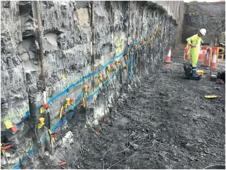
Fig.7.Geophones attached to the face using angle-iron brackets screwed directly into the rock face.

The semi-permanent monitoring network consisted of four side-view sensors(two in each borehole)installed in the boreholes located 5 m behind the excavated face.These were repositioned after each excavation cycle to the new excavation depth,with builtin clamps coupling the instruments to the borehole casing.The borehole sensors contribute an important role in improving the event location precision and detection limit,which is of great importance when aiming to estimate the extent of disturbance away from the face.

Rock face sensors were installed following each excavation cycle,which ultimately created a network of 21 sensors across the excavated face.Prior to the application of shotcrete after each excavation,and while the slope face was still exposed,the rock surface was smoothed to ensure good coupling to the sensor.A protective duct was then installed to provide access after the shotcrete application.Once the shotcrete had been sprayed,the instruments were mounted inside the ducts,using the housing in the duct to clamp the instrument firmly to the rock face.After each excavation lift,additional rock-face sensors were installed that ultimately created a network of 21 sensors.

AE sensors measure motion predominantly in the direction normal to the sensor face,however,they are also sensitive to a smaller amount of perpendicular (approximately -15 dB at 90°and -10 dB at 160°incident) and backward motion as well(Manthei et al.,2001).There are,however,currently no triaxial AE instruments existing today which operate within this frequency and sensitivity range.Accordingly,sensors were oriented such that the component of motion measured was perpendicular to the rock face,i.e.in the direction where events were expected to occur.In other words,the sensors were optimally oriented to detect P-wave particle motions,although in many cases,clear S-wave arrivals were also visible.

Continuous data were acquired by this sensor network between 15 August 2017 and 31 January 2018,with the exception of the times when the active surveys were being acquired and the borehole sensors were repurposed for these surveys.A real-time triggering algorithm was used during the passive monitoring to detect potential seismic events,with waveforms recorded when a specific amplitude threshold was crossed on at least two sensors.Some site activities (such as nailing and dowel installation) and stormy weather produced large numbers of triggers.As an example,on 14 December 2017,there were more than 185,000 triggers,which were caused by cables blowing against the rock face during a period of strong winds.To further improve the quality of the dataset,we apply a second tiggering algorithm to the real-time dataset using the short-term average/long-term average (STA/LTA) method,which is parameterised with a 0.1 ms STA and 0.3 ms LTA window length and an STA/LTA detection threshold of 8.

Separating genuine AE events (i.e.events produced by stress release and fracturing in the rock mass)from both human activities(drilling,excavating,nailing etc.) and natural noise proved challenging.We analysed the period between 21 September 2017 and 31 January 2018,with the start of this period representing the date when at least five sensors were installed on the rock-face.To ensure that events associated with onsite human activities were not used,we also restricted our analyses to times when no work was taking place on the site.For most of the operational periods,this corresponded to times of 2-6 a.m.Additionally,a Christmas shutdown between 22 December 2017 and 2 January 2018 was used,since no work took place at the site during this period.Fig.10 illustrates the data selection quality control (QC) criteria we adopted during the project.

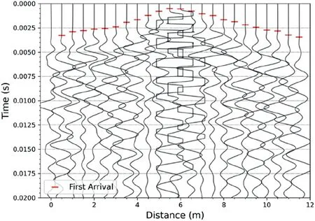
Fig.8.Example waveforms recorded from a single shot,with the first breaks picked manually.

The waveforms for events identified by the triggering algorithm were manually inspected,with P-and S-wave arrival times being picked where it was possible to identify clear arrivals from each trace.This conservative approach was adopted to ensure high fidelity in the travel time dataset.An example of waveforms from one of these AE events is shown in Fig.11.Event locations were inverted from the observed P-wave(and where identified,S-wave)arrival times,with the best-fit location computed using an Eikonal solver (Lomax et al.,2012) based on the velocity model derived from the cross-well observations previously described.We incorporate the excavation related disturbance into the model by including the velocity reduction within the initial 1-2 m of the rock face imaged by the active surveys.Disturbance will primarily influence rock face sensor measurements and not including this velocity reduction would result in an overestimation of the event’s distance into the rock mass.The final criteria applied to our picoseismic event population is that only events with location uncertainties (90% confidence interval) lower than 1.5 m in the N,E,and Z coordinates were included in the final dataset.

In total,199 such AE events were identified,which is significantly lower than that observed in other studies situated in more favourable,less attenuating rock environments (Manthei and Plenkers,2018).The locations of these events are predominantly clustered within 3 m of the face,and increase in depth with time,indicating that events are occurring near to recently excavated rock(Fig.12).We estimate the mean location error to be 0.95 m into the rock mass(east)and 0.7 m in both the north and vertical direction.Fig.13 shows a histogram of the event occurrence rate.While there is some clustering around periods of excavation and trimming,events also occur when no activities are taking place (for example during January 2018).An interesting linear cluster of events was observed between the elevations of 7-12 m located near the former borehole S3,which was sealed with concrete then partially destroyed during excavations.This seismic cluster may relate to stress changes and damage caused the creation of the borehole or surface noise transmitted into the rock mass by the borehole.Either way,this partially explains an increase in events during the middle of October.Excluding this cluster,we observed a low number of events that occurred relatively irregularly within the rock mass.While events occurring during excavation may not be captured due to high noise levels and the spatial resolution of the array,when the network was expanded,we have not observed a significant pattern of events.This implies that rock damage is created during and immediately after the excavation period.

3.2.1.Network spatial resolution

Any interpretation of the passive monitoring must consider with detection limits,which can be expressed as the spatial volume in which we would expect the array to be able to reliably detect events of a given magnitude.We found that over 90% of the AE events occurred within 3.2 m from the rock face,which raises the question of whether this limit defines the extent of the excavation disturbance,or if it is simply a consequence of the monitoring network limitations,since most of the sensors were installed on the rock face.Whereas passive recordings of picoseismicity from distances >200 m are documented in hard rock or salt rock environments (e.g.Plenkers et al.,2010;Philipp et al.,2015),the detectability distance can be limited to a few metres in soft rock environments(Le Gonidec et al.,2012).As there are no comparable case studies carried out in a similar geological setting as those carried out at HPC,it is difficult to estimate the likely spatial completeness from literature alone.It would however be expected that the detectability limits and the extent of rock disturbance may be somewhat similar,therefore,a more quantitative assessment is required.

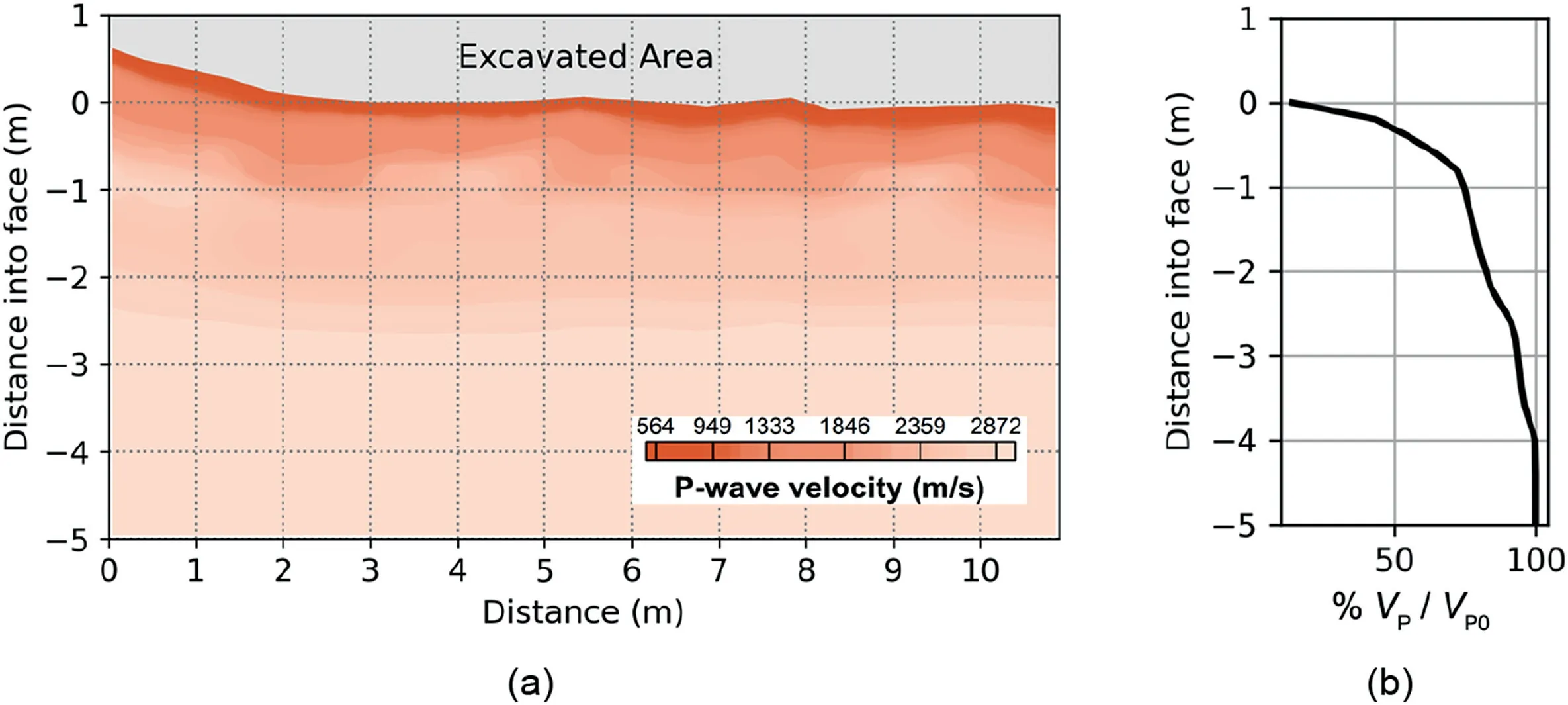
Fig.9.(a) Tomography model of velocity variations into the excavated rock mass (mapview).(b) Observed velocity as a percentage of the baseline values,with 50% reduction occurring in the initial 0.5 m of the slope face.

In order to address this question,we assessed the maximum detectability distance of each sensor and then translated these distances into network detectability limits.The approach is similar to that adopted by Plenkers et al.(2011),though we were unable to incorporate the magnitudes into the assessment as the amplitude response of the piezoelectric sensors was uncalibrated and amplitudes were heavily influenced by the nature of the instrument coupling.We generally assume events share a common source mechanism with an equivalent rupture area/magnitude.However,significant outliers were present on several sensors which may relate to larger amplitude events that would be detectable at greater distances (see Fig.14a).To ensure estimated detectability limits were unaffected by these outliers,we computed cumulative probability distribution and selected the 90% confidence value as the maximum detectability distance of a sensor(see Fig.14b).These estimates reflect both the surrounding rock properties and the performance of the individual sensors.Detectability distances of the rock face sensors generally increase with depth,with shallower sensors achieving 5-6 m increasing to around 7 m further down the excavation slope.Borehole sensors have slightly higher detectability distances.Given their location within the rock mass,we might expect these sensors to experience lower levels of noise.Several sensors performed poorly,possibly due to poor coupling to the rock face or instrument malfunction,and these had lower detectability distances or were excluded from the assessment.

For each excavation period,we determined the spatial variation in detectability for the network inplace at that time using the calculated detectability distances.From these distances,we determine regions within the rock mass where at least five sensors are capable of recording an event;five sensors are the minimum station threshold adopted in the event selection criteria.The detectability regions are presented in Fig.15 and show that the network is generally able to identify events within 5 m of the rock face,which are broad in agreement with the spatial resolution observed by Le Gonidec et al.(2012).As the number of sensors increased,the spatial resolution improved until excavation cycle 5,when two poorly performing sensors had a detrimental effect on the spatial resolution.For all excavation cycles,the resolution distance exceeds the 3.2 m region fromthe rock facewhere 90%of the AEevents occur.Thissupports the conclusionthatthespatialdistribution of AEeventsreflectstheextent of disturbance within the rock mass and not limitations of the network.

4.Discussion

Fig.10.Data processing workflow for the picoseismic data.To ensure that only genuine picoseismic AE events were identified,only events detected on at least 5 sensors during periods with no site activity were considered.

Both geophysical approaches employed in this study have detected excavation related damage within the rock mass.Broadly they agree that the maximum extent of disturbance is about 3 m from the rock face;P-wave velocities return to their background values at about 3 m,while over 90%of the AE events occur within 3.2 m.The observed extent of the AE events is not constrained by the detectability limits of the array,which has been assessed as at least 5 m into the rock mass when requiring an event to be recorded on five or more sensors.There is a noticeable difference between the shapes of the distribution curves derived from the two methods(see Fig.14),with seismic tomography revealing an exponential decay in velocity perturbation into the rock face,but a more linear progression was observed with the AEs.This results in P-wave velocities returning to 50%of their background values within 0.5 m of the rock face,while 50% of AEs occur within 1.6 m (see Fig.16).These differences likely reflect differences in the physical mechanisms being assessed in each survey and are comparable to the laboratory results of Nihei and Cook (1992).Seismic velocities are significantly reduced by the opening of fractures resulting from a decrease in confining pressure,with velocity reduction most severe at the rock face.In contrast,AEs are generated by the rapid release of elastic energy relating to crack growth or deformation within the rock mass,and are generally more evenly distributed within the region of disturbance.However,fewer events occur within the immediate area of the rock face,where higher rock disturbance and lower confining pressures are encountered.This decrease in the number of events therefore suggests there is insufficient stress imposed on fractures to produce AE detectable events in regions on significant rock disturbance.

Fig.11.Example waveforms from a AE event.Sensor numbers are indicated in the top-left corner of each plot(1-4 are borehole sensors,5-15 are rock-face sensors).P-wave arrival times are indicated by the red lines,and S-wave arrivals by the dark-blue lines.Unclear arrivals were not included to ensure a high-fidelity dataset.

As this is the first known application of this method in this shallow geological setting it is difficult to directly compare the event population to other studies,however the number of events is significantly lower than that of similar studies performed in deep mines,where confining pressures are much higher (Manthei and Plenkers,2018).This may indicate that rock disturbance occurs during or very shortly after slope excavations,or that at lower confining pressures,much of the disturbance takes place in an aseismic manner.

The recording of seismic events within the excavated slopes of HPC on picoseismic scale is a significant achievement,and the locations of these events correlate with the extent of P-wave velocity changes observed in active seismic methods.These seismic events have a dominant energy in the frequency range from approximately 1 kHz-10 kHz,which means,following Kwiatek et al.(2011),Naoi et al.(2014),and Kwiatek et al.(2018),that they correspond to either shear fractures triggered by excavation or newly generated fractures potentially with tensile opening on the cm-or dm-scale,i.e.in the magnitude range of -4

Fig.12.Locations of 199 AE events passing QC criteria.Orange triangles show the final sensor locations,coloured dots show event locations (coloured by occurrence time).The greyed area represents the rock mass and the white area shows the excavated areas.

Fig.13.Histogram of 199 AE events passing the QC criteria recorded between 21 September 2017 and 31 January 2018.The start of this period represents the date when more than 5 sensors were installed on the rock face,which occurred after the second excavation lift.

A major challenge relating to the processing of the passive dataset is differentiating between fracturing induced events and noise events generated by site activity.This may be a result of the high levels of seismic attenuation present within the shallow subsurface,which significantly reduces the frequency of the recorded AE events.It is therefore difficult to identify fracture induced events based on their frequency content,and to ensure dataset fidelity,that is only events during site inactivity were included.Future studies that incorporate developments in machine learning may prove more successful at identifying events during noisier periods of site activity(e.g.Bergen et al.,2019),however,this is beyond the scope of this study.

When evaluating the recorded picoseismic events,it is important to note that the magnitude of the events is unknown.As described extensively in literature (e.g.Manthei and Plenkers,2018),in situ AE sensors are uncalibrated,which poses significant limitations on the magnitude estimation.Whereas in some hard rock environments it was possible to extract true magnitudes by calibrating the AE sensors onsite,this approach was not possible at HPC.Being unable to calculate true magnitudes is a major short coming of the in situ AE monitoring technique.In the future,we hope that better calibrated AE sensors will become available.Nonetheless,even without a precise calculation of the event size,we find that the temporal-spatial observation of the events alone provides important information about the processes inside the rock volume,which cannot be retrieved by any other method.

P-wave velocities,which are directly relatable to rock strength(e.g.Chang et al.,2006),were observed to exhibit the same exponential change as proposed by the velocity-pressure model of Ji et al.(2007).This suggests that while AEs provide a temporal measurement of rock disturbance,the spatial extent is best assessed in soft rock environments using seismic tomography.Following a similar approach proposed to estimate RQD(McDowell,1993),we relate seismic velocities to disturbance through defining D as the ratio between the post-excavations velocities (Vp) and baseline values (Vp0).The change in Vpreflects the severity of the disturbance,and therefore Vp/Vp0provides an assessment of rock disturbance,D.In order to relate the velocity ratio to the rock disturbance,we include the parameter D0,which is the visual site assessment of disturbance at the rock face.Thus,we propose

where the constant,a,allows for future refinement of the relationship based on laboratory analysis.Ideally,this relationship should be estimated prior to excavations,which could be achieved through the incorporation of the velocity-pressure model of Ji et al.(2007)(Eq.(6)).This would require a recalibration of the relaxation term,B,and the decay constant,k,for specific near-surface lithologies and an accurate measurement of confining pressure,which is not feasible with this dataset alone.

5.Conclusions

Fig.14.Source-receiver distances for network sensors:(a)individual measurements recorded on 21 sensors (circles)and detectability limits(red lines).Sensors 1-4 are borehole instruments,while 5-21 are located on the rock face with the larger ID numbers located towards the base of the excavated slope.Poorly performing sensors either had lower detectability distances(e.g.sensors 3)or were excluded from the assessment(e.g.sensors 19,20 and 21);and(b)example cumulative probability distributions for sensors 6,12,and 18 located at varying depths below ground level (b.g.l.).The 90% confidence interval was used as the sensor detectability distance to remove significant outliers.

Fig.15.Detectability distances for periods after excavation cycles 2-5.The network is generally capable of recording event within 5 m of the rock face.(a)Lift 2:4 m b g.l.;(b)Lift 3:8 m b g.l.;(c) Lift 4:11 m b g.l.;and (d) Lift 5:14 m b g.l.

Fig.16.Cumulative proportion of AE events(red)as a function of distance into the face compared with the average measured velocity profile (black).Velocity returns to 90%of the undisturbed value within 2 m,while 90%of the AE events occur within 3.2 m of the excavated face.

Excavation related damage has been imaged through a combination of passive and active seismic methods at HPC,with both approaches indicating that disturbance is limited to within approximately 3 m of the rock face.Seismic velocities reveal an exponential decay in disturbance into the rock mass,with the majority of the damage occurring within the first 0.5 m.A small number of picoseismic events have been recorded with no clear relationship to periods of excavation.While events which occur during excavation may not have been recorded due to high noise levels or the spatial resolution of the network,that absence of events after the network has been expanded implies disturbance occurs during or immediately after excavation stages.At HPC,seismic velocities are therefore considered to represent a good proxy for rock disturbance,and relationship between disturbance and P-wave velocity is based on a ratio of the measured and baseline velocities.Monitoring picoseismicity adds confidence to our interpretation of the extent of the disturbance zone,but we note that such passive seismic monitoring is difficult in noisy excavation environments.

The visual observations of joint aperture and the number of random joints,from the logging of faces,indicated that new joints had not been formed and dilation of existing joints was small (the majority of joints being recorded as tight in the rock descriptions for the excavated faces).The corresponding assessment of the level of disturbance based on the excavated faces,with reference to the published data on level of disturbance,indicated that the level was at most between 0.1 and 0.2,when using a rock wheel to trim the slopes.

By determining the extent of the disturbance in excavations for Unit 1,through the use of the geophysical surveys,a better understanding of the likely reduction in rock mass strength was obtained.The information provided by the geophysical surveys enabled a reassessment of the excavation process,and a simplified methodology,without the use of vertical dowels,was adopted for subsequent excavations at both Units 1 and 2.This resulted in a corresponding reduction in the construction programme of approximately three to four weeks and a significant reduction in construction costs.

At sites where understanding the strength of the rock mass is critical(e.g.large dams,deep caverns for nuclear waste storage,or nuclear power stations),the survey methods described in this paper could be used to give better engineering certainty on a critical design parameter,D,and as a result could lead to a reduction in both construction costs and programme.The results of these seismic surveys led to a redesign of the excavation strategy at HPC.As the rock disturbance was not as severe in terms of depth into the slope,it was concluded that the installation of vertical dowels was no longer required.Ultimately,such geophysical surveys have the potential to better inform excavation strategies and therefore reduce engineering or excavation costs in large projects,such as the construction of nuclear power plants or large-scale tunnel projects,like the proposed High Speed 2 railway link in the UK.

Declaration of competing interest

The authors declare that they have no known competing financial interests or personal relationships that could have appeared to influence the work reported in this paper.

Acknowledgments

The work was funded by EDF energy,who we also thank for providing us the permission to publish,and Bristol University Microseismic Projects (www1.gly.bris.ac.uk/BUMPS/).We thank Pete Johnson and Lee Appleby for their support and securing funding for the project.The authors would also like to express our gratitude to the project engineers and site personnel who helped install and maintain the seismic monitoring network,specifically Chris Bent,Keith Todd and David Lindfield from Kier/BAM JV.