Multi-geomagnetic-component assisted localization algorithm for hypersonic vehicles*

Kai CHEN，Wen-chao LIANG，Cheng-zhi ZENG，Rui GUAN

1School of Astronautics,Northwestern Polytechnical University,Xi’an 710072,China

2China Aerodynamics Research and Development Center,Mianyang 621000,China

Abstract:Owing to the lack of information about geomagnetic anomaly fields，conventional geomagnetic matching algorithms in near space are prone to divergence.Therefore，geomagnetic matching navigation algorithms for hypersonic vehicles are also prone to divergence or mismatch.To address this problem，we propose a multi-geomagnetic-component assisted localization (MCAL)algorithm to improve positioning accuracy using only the information of the main geomagnetic field.First，the main components of the geomagnetic field and a mathematical representation of the Earth’s geomagnetic field (World Magnetic Model 2015) are introduced.The mathematical relationships between the geomagnetic components are given，and the source of geomagnetic matching error is explained.We then propose the MCAL algorithm.The algorithm uses the intersections of the isopleths of the geomagnetic components and a decision method to estimate the real position of a carrier with high positioning accuracy.Finally，inertial/geomagnetic integrated navigation is simulated for hypersonic boost-glide vehicles.The simulation results demonstrate that the proposed algorithm can provide higher positioning accuracy than conventional geomagnetic matching algorithms.When the random error range is ±30 nT，the average absolute latitude error and longitude error of the MCAL algorithm are 151 m and 511 m lower，respectively，than those of the Sandia inertial magnetic aided navigation (SIMAN) algorithm.

Key words:Geomagnetic navigation;Isopleth;Geomagnetic components;Integrated navigation;Kálmán filter

1 Introduction

Near space is different from aviation and aerospace fields:near-space altitude ranges from 20 to 100 km (Lv et al.，2017;Wang WK et al.，2019).Compared with conventional aviation space，near space provides richer task modes and faster communication (Dong et al.，2019).Hypersonic vehicles have advantages such as high speed，wide range (Li et al.，2019)，fast response，strong capability for aviation and space operations，and good stealth performance，giving them strategic significance and prospects for broad military applications (Chen et al.，2017;Wang YY et al.，2019;Xia et al.，2019;Yang et al.，2019).

The navigation of hypersonic vehicles is based mainly on inertial navigation systems (INSs).The global navigation satellite system (GNSS) is used as an auxiliary navigation method to correct the cumulative error of the INS (Hu et al.，2019).However，the GNSS is not an autonomous navigation system，and is sensitive to interference (Wei et al.，2018).When applying this system to hypersonic vehicle navigation，other problems include signal loss and carrier phase lock issues.The application of inertial/celestial integrated navigation to hypersonic vehicles remains in its infancy.In addition，the temperature field of hypersonic vehicles in flight is strongly influenced by the complexity of the thermal environment (Shen et al.，2020)，such as ambient temperature，air flow，aerodynamic heating effects，and solar radiation，resulting in temperature gradients within the optical system.These factors affect the geometry and performance of the airborne optical components.Geomagnetic navigation has recently been adopted as a passive navigation method.This system has advantages，such as strong stealth capability and good adaptability，and it can also overcome the error accumulation problem observed in INSs over time(Chen et al.，2018;Wang and Zhou，2019).A geomagnetic navigation system can provide carriers with all-weather，all-day，all-region navigation services(Goldenberg，2006;Wang and Zhou，2019;Xiao et al.，2020).

Many algorithms using geomagnetic positioning or navigation have been proposed or verified in recent years.Duan et al.(2019) proposed a novel inertial/geomagnetic integrated navigation algorithm based on a matching strategy and hierarchical filtering.Through the evaluation of the distribution of magnetic measurements，several controllable magnetic values are regenerated to participate in the geomagnetic matching algorithm.Then，based on the hierarchical filtering strategy，the integrated navigation filter is designed.The novel algorithm overcomes the inability of traditional geomagnetic matching algorithms to provide continuous，real-time navigation information.At the same time，the accuracy of the inertial/geomagnetic integrated navigation algorithm is improved.Li et al.(2017) proposed a multiobjective evolutionary algorithm applicable to autonomous underwater vehicles (AUVs).Inspired by biological navigation behavior，this algorithm can overcome the loss of AUVs in the navigation phase owing to extreme values in abnormal geomagnetic regions (Section 2.1).Simulation results demonstrated the reliability and feasibility of the proposed approach in complex environments.Wang JH et al.(2019) proposed a novel matching algorithm called the multi-parameter matching model of the least magnetic distance (MPMD) algorithm.The algorithm matches the magnetic eigenvector product of the total geomagnetic field and the geomagnetic component，based on Euclidean distance.Underground geomagnetic positioning using the MPMD algorithm was tested and compared with other algorithms in nine tunnels in a mine.Simulation results showed that the new algorithm has the advantages of high positioning accuracy and strong anti-noise capability.This algorithm is suitable for underground spaces with complex geomagnetic distributions.Chen et al.(2018)proposed a new geomagnetic navigation method based on a vector matching algorithm，namely vector iterative closest contour point (VICCP).This algorithm combines the searching principle of trusted point sets and performs tracking with the matching principle of geomagnetic vector correlation restriction.In simulation experiments，the positioning error of VICCP was found to be less than that of iterative closest contour point (ICCP) under the conditions of nonobvious scalar geomagnetic features.This result was also verified in physical experiments.He et al.(2019) developed a combined orientation compass based on polarized skylight/geomagnetism/micro inertial measurement unit (MIMU) information.The heading angle information is extracted from the geomagnetic information and input into the Kálmán filter together with the two other types of information.After fusing the three types of orientation information through the Kálmán filtering algorithm，the orientation accuracy was found to be better than 0.5° in vehicle experiments without satellite signals.

Since near space is far from the crust，the crustal magnetic field is almost negligible，and only the main geomagnetic field can be used as the navigation magnetic field (Zong et al.，2018).Change in the main geomagnetic field is relatively gradual.Owing to the high speed and wide flying range of hypersonic vehicles，it is difficult to attain the required navigation accuracy using conventional geomagnetic sequential matching algorithms such as the magnetic contour matching (MAGCOM) algorithm，or recursive filtering algorithms such as the Sandia inertial magnetic aided navigation (SIMAN) algorithm.In some cases，even mismatches may occur.To correct the divergence or mismatch of geomagnetic navigation，in this study，we analyze the main geomagnetic field and the source of error in the geomagnetic matching navigation system.We propose a multi-geomagneticcomponent assisted localization (MCAL) algorithm，in which a geomagnetic field with multiple geomagnetic component features is used to estimate the true position of a carrier through multiple geomagnetic component isopleths.This can ensure accurate positioning of hypersonic vehicles.

The remainder of this article is organized as follows:Section 2 introduces the composition of the geomagnetic field，mathematical formulations of the main geomagnetic field model，and the source of geomagnetic matching error.Section 3 presents the MCAL algorithm developed in this study.Section 4 reports the results of an integrated navigation simulation experiment.

2 Geomagnetic field and geomagnetic matching error

2.1 Geomagnetic field

The geomagnetic field is a magnetic field generated inside the Earth and is a naturally occurring geophysical field (Hu et al.，2019).It is composed mainly of a geomagnetic field，geomagnetic anomaly field，and perturbed magnetic field.The main geomagnetic field accounts for more than 95% of the total geomagnetic field，and is the primary component of the Earth’s magnetic field，varying gradually with time.The geomagnetic anomaly field is a secondary magnetic field caused by the magnetization of crustal rocks，and is also known as the crustal magnetic field.It exists mainly in the space around the crustal rocks.The perturbed magnetic field is a disturbed magnetic field caused by solar activity，varying drastically with time (Heimpel and Evans，2013).The geomagnetic field can be expressed as (Liu et al.，2019)

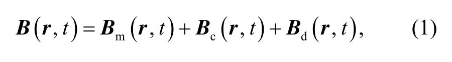
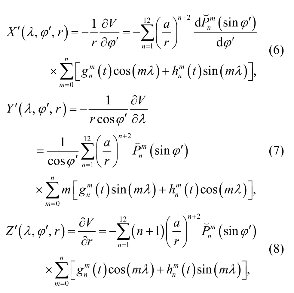
whereBm(r，t) represents the main geomagnetic field，Bc(r，t) represents the crustal magnetic field，andBd(r，t) represents the perturbed magnetic field.ris the position vector，andtis the time.For near-space hypersonic vehicles，the strength of the crustal magnetic field in near space is almost negligible，and the perturbed magnetic field can be categorized under the disturbed magnetic field.Hence，hypersonic vehicles are navigated only through the main geomagnetic field.The main geomagnetic field can be expressed as a negative spatial gradient of the magnetic scalar potential，which can be represented by the following geocentric coordinate system (Chulliat et al.，2015):whereλrepresents the longitude，φ′represents the geocentric latitude，rrepresents the radius，andVis the scalar potential.To expand the above formula according to the spherical harmonic function，we have

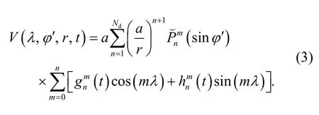
In the Earth’s geomagnetic field model (World Magnetic Model 2015 (WMM2015))，the expansion orderNdis 12，ais the geomagnetic reference radius，andare the time-related Gaussian coefficients at timet.represents the Schmidt semi-normalized associated Legendre function of degreenand orderm，formulated as follows:

whereμis the argument of the function.

The geomagnetic componentsX′，Y′，andZ′ in the three directions (north，east，and down) can be expressed in the geocentric reference system as:which can be obtained by substituting in the above formula the values ofX，Y，andZgeomagnetic components at a certain coordinate (λ，φ′，r).

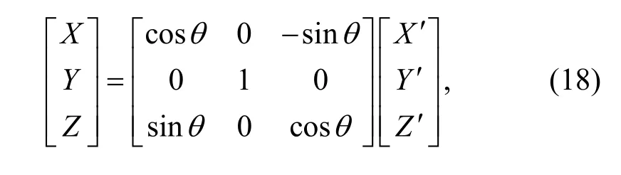
Given the actual navigation requirements，the coordinates are converted to the geodetic coordinate system (λ，φ，h)，whereφis the geographic latitude，andhis the height above WGS-84 ellipsoid.Fig.1 shows the coordinates of pointPin different coordinate systems.

Based on the geometric relationships in Fig.1，the spherical coordinates can be converted to rectangular coordinates:

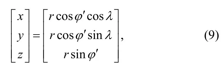
wherex，y，andzare the coordinate values of pointPin the geodetic rectangular coordinate system.Thus，the geodetic rectangular coordinates can be converted to the geodetic coordinates:

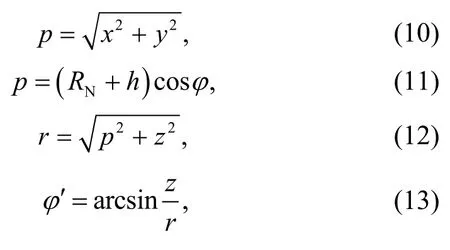
wherepis the horizontal projection of radiusrshown in Fig.1.RNis the normal radius，andcan be expressed as

whereawis the semi-major axis given by WGS-84，andaw=6 378 137.0 m.eis the eccentricity of the ellipsoid，ande==0.08181919，wherefis the flatness given by WGS-84.

Hence，X′，Y′，andZ′ can be converted to the ellipsoid reference system through the above relationship as:

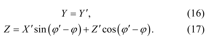
This can be presented in the form of a direction cosine matrix:

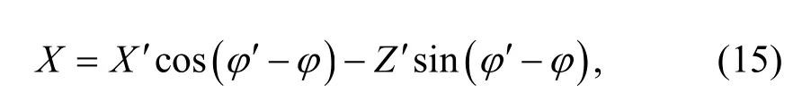
whereθ=φ′−φ.

To describe the spatial distribution characteristics of the geomagnetic field，the main geomagnetic field vectorBm（λ，φ，h，t）is expressed using seven geomagnetic elements (F，H，X，Y，Z，D，andI) in the north–east–down (NED) coordinate system.Fig.2 shows a schematic of the geomagnetic elements，including the definitions and symbols of each.

Fig.1 Point P in different coordinate systems ωe is the Earth’s rotation rate

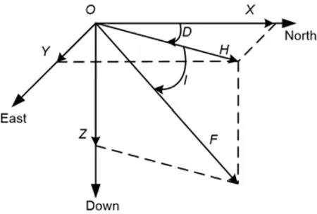
Fig.2 Schematic of geomagnetic elements

The following are the conversion relationships between the geomagnetic components:

Fig.3 shows the total intensity distribution of the geomagnetic field in the WMM2015 model，and Fig.4 shows its isopleth distribution.

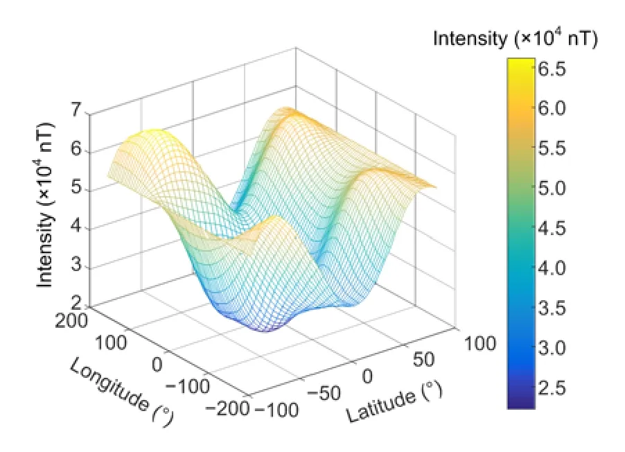
Fig.3 Total intensity distribution of the geomagnetic field in the WMM2015 model

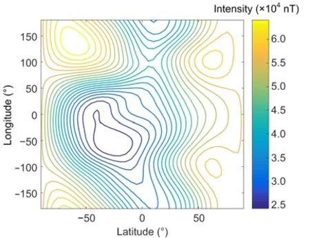
Fig.4 Total intensity isopleth distribution of the geomagnetic field in the WMM2015 model

2.2 Source of geomagnetic matching error

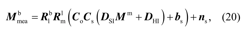
Geomagnetic matching errors in near space arise mainly from two sources:the measurement error when the geomagnetic field is measured，and the model error between the main geomagnetic field reference map (generated by WMM2015) stored in the navigation computer and the real magnetic field(Fig.5).

In Fig.5，Mmearepresents the measured geomagnetic field value，Mprarepresents the practical geomagnetic field value，andMmaprepresents the reference map of the main geomagnetic field.There is a measurement error betweenMmeaandMpra，and a model error betweenMpraandMmap.The error betweenMmeaandMmapis a mixed error induced by the overlay of the two previous errors.

A three-axis strapdown magnetometer measurement model can be expressed as follows (Song et al.，2016):

The errors of the main geomagnetic field model can be categorized into two types:commission errors and omission errors (Chulliat et al.，2015).Commission errors can be attributed to inaccurate model coefficients.Omission errors can be attributed to the lack of representation of the crustal magnetic field in the main geomagnetic field model and some shortterm magnetic field changes due to natural phenomena，such as geomagnetic storms (Harsha and Ratnam，2020).Therefore，the error in the main geomagnetic field value varies with time and has a strong uncertainty.In this study，we mainly analyze the positioning accuracy and robustness of the geomagnetic matching algorithm.Hence，a uniformly distributed random variable is applied to represent the mixed error induced by the overlay of the sensor error and main geomagnetic field model error.

3 MCAL algorithm

3.1 Principles of the algorithm

During the movement of a carrier，the geomagnetic field value is measured in real time using three-axis magnetic sensors installed on the carrier.When the mixed error is not considered，a matching area with a size of 3σx×3σyis selected on the basis of the position information output by the INS，whereσxis the maximum error in thexdirection of the INS，andσyis the maximum error in theydirection.The geomagnetic reference map information of the matching area is extracted based on the magnetic measurement value of the sensors to plot the corresponding isopleths.When there is no error between the measured and reference geomagnetic field values(i.e.when the mixed error is 0)，the intersection of these isopleths is the true position of the carrier (Li，2013).Fig.6 shows a schematic of the algorithm.

The seven geomagnetic elements of the geomagnetic field can be divided into two categories in terms of their characteristics:one based on the intensity，and the other based on the angle.In this study，we used three mutually orthogonal intensity componentsX，Y，andZas the matching characteristic parameters.When a carrier moves，the three-axis magnetic sensor can measure the geomagnetic field value in the three-axis direction at the position of the carrier.The measured value is subjected to coordinate conversion to obtain the component values in the north，east，and downward directions in the NED coordinate system.Based on the measured geomagnetic components，the geomagnetic isopleth corresponding to this value and the coordinates of each point on the isopleth can be found in the geomagnetic reference library.The position of the carrier should be located on the three isopleths simultaneously.In other words，the intersection of the three geomagnetic component isopleths is the optimal estimate of the true position of the carrier.

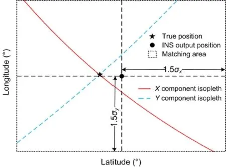
Fig.6 Schematic of the algorithm

Notably，the three geomagnetic isopleths have a complicated intersection pattern.On the one hand，because the measurement errors of the three-axis magnetic sensor and model errors cannot be 0 (i.e.the mixed error cannot be 0)，the three isopleths may not intersect at the same point.Moreover，the number of intersections is likely to be greater than 1.On the other hand，since the geomagnetic isopleths may have arcs with large curvature or relatively complex curves，and may overlap with each other，this could lead to multiple intersections.Hence，to ensure real-time positioning，the isopleths of the first two components are obtained first.If the intersection number of the isopleths of the two components isN≥2 orN=0，the isopleth of the third component is then introduced to make the decision.At the same time，the matching area needs to be divided on the basis of the position solved by the INS，and the mixed error range estimated by the geomagnetic assisted navigation system.Fig.7 shows the condition with mixed errors and when the isopleths have multiple intersections.

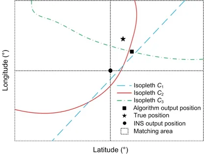
Fig.7 Schematic of multiple intersections with mixed error

The following are the steps involved in the integrated navigation algorithm:

1.The values of the two geomagnetic components (e.g.XandY) measured by the magnetometer at the position of the carrier are recorded asM1andM2.The length of the matching area can be calculated by

whereLrepresents the length of the matching area，hxandhyare the slopes of the geomagnetic value in thexandydirections，respectively，and Erreis the maximum mixed error (unit:nT) estimated by the geomagnetic assisted navigation system.For two or three geomagnetic components，obtainLand take the maximum value.

2.The geomagnetic reference library data carried by the carrier are read，and the isopleths corresponding toM1andM2in the matching area are plotted asC1andC2，respectively.

3.Nrefers to the number of intersection points ofC1andC2.IfN>1，the third geomagnetic component(e.g.Z) valueM3is introduced，and its corresponding isoplethC3is drawn.The distances between all the intersection points are calculated，and the mean value of the intersection coordinates of the closest intersection cluster is selected as the matching result output;ifN=1，the intersection point is taken as the matching output;ifN=0，the INS output is regarded as the matching output and the Kálmán filter in step 4 is skipped.

4.The difference between the matching results and the INS output position is taken as the input of the Kálmán filter and its filtering result is the final output.

Fig.8 shows the flowchart of the MCAL algorithm.

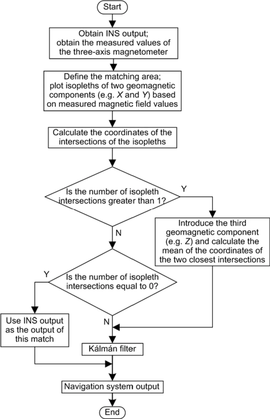
Fig.8 Flowchart of the MCAL algorithm

3.2 Kálmán filter

The state equation and observation equation of Kálmán filter are:

whereX(t) is the error state variable of the system developed，F(t) is the system state transfer matrix，G(t) is the noise transfer matrix，W(t) is the white noise error matrix，Z(t) is the observation vector，H(t)is the observation matrix，andV(t) is the observation noise matrix of geomagnetic matching.For more details about the Kálmán filter，please refer to Chen et al.(2020a).

4 Simulations

In this study，we used the WMM2015 model (Qi et al.，2017;NCEI，2019) to generate a geomagnetic reference map:the altitude was 25 km，latitude ranged from 40° north latitude to 48° north，longitude ranged from 109° east longitude to 112° east，and grid resolution was 0.01 (°)/div.Interpolation processing was applied to the geomagnetic map，and a grid resolution of 0.00125 (°)/div was achieved.Fig.9 shows the flight trajectory of the hypersonic vehicle in the simulation experiment.The launch point and yaw of the flight trajectory were set randomly.

The flight of hypersonic boost-glide vehicles in near space can be divided into different phases:a boost phase，free ballistic phase，ballistic re-entry phase，ballistic pull-up phase，and equilibrium gliding phase (Chen et al.，2019).In this study，we analyzed the geomagnetic navigation problem only in the cruise phase，so the trajectory was simplified.It was assumed that the aircraft accelerated，climbed，cruised at a constant speed，turned left，turned right，and performed other movements in sequence during the entire flight.The simulation time was 790 s.Fig.10 shows the ballistic trajectory.

The equilibrium gliding phase of hypersonic vehicles in near space was modeled by a navigation simulation.The cruising speed of the aircraft was 2000 m/s.The simulation time was 790 s，during which the aircraft was flown only by INS navigation for a period of 0–420 s，and by inertial/geomagnetic integrated navigation for the remaining period.The sampling time interval of the geomagnetic magnetic sensor was 1 s，the inertial navigation solution period was 0.01 s，and the Kálmán filter period of the integrated navigation was 1 s.During quiet periods of the geomagnetic field，the disturbance storm time index is between +20 and −20 nT (Cui et al.，2020).Therefore，the random error ranges of the mixed error were set to±0.1，±1，±5，±10，and ±30 nT.The MCAL algorithm was simulated.The results were compared with those of the MAGCOM algorithm with heading angle correction，ICCP algorithm，and SIMAN algorithm.Table 1 lists the parameters for the strapdown inertial navigation system (SINS) (Chen et al.，2020b).Figs.11–15 show the positioning errors.Table 2(p.366) lists the average absolute error when inertial/geomagnetic integrated navigation was used for the period of 420–790 s.

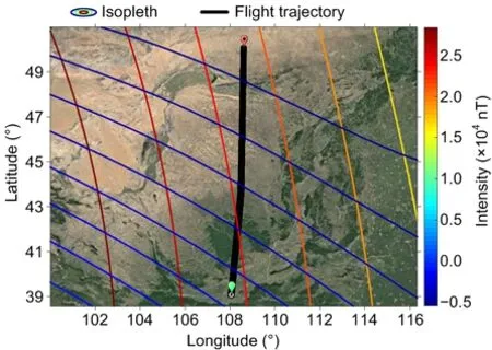
Fig.9 Flight trajectory in simulation

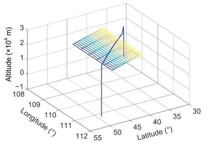
Fig.10 Simplified trajectory and geomagnetic navigation area of a near-space hypersonic vehicle

Table 1 Parameters for the SINS (Chen et al.,2020b)

The absolute average error listed in Table 2 was calculated using the following equation:where Errirefers to the difference between the true position and the integrated navigation output position，Trepresents the duration of the integrated navigation(the geomagnetic navigation interval was 1 s)，andErefers to the absolute average error.The algorithm running time was obtained through simulation on the same computer with a mixed error range of ±10 nT.

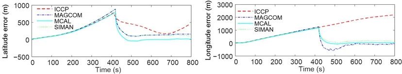
Fig.11 Integrated navigation error for a magnetic error range of ±0.1 nT

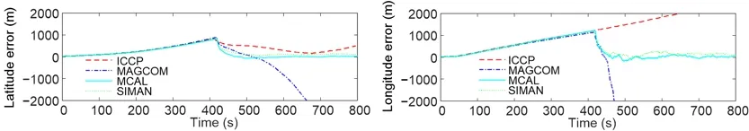
Fig.12 Integrated navigation error for a magnetic error range of ±1 nT

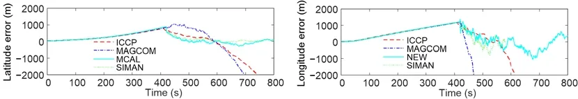
Fig.13 Integrated navigation error for a magnetic error range of ±5 nT

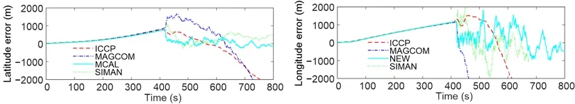
Fig.14 Integrated navigation error for a magnetic error range of ±10 nT

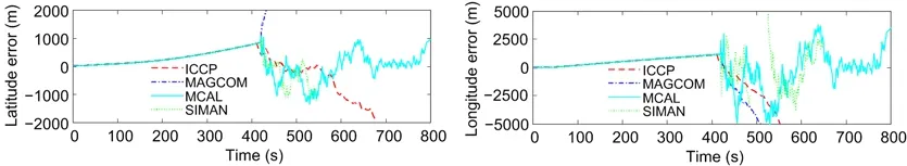
Fig.15 Integrated navigation error for a magnetic error range of ±30 nT

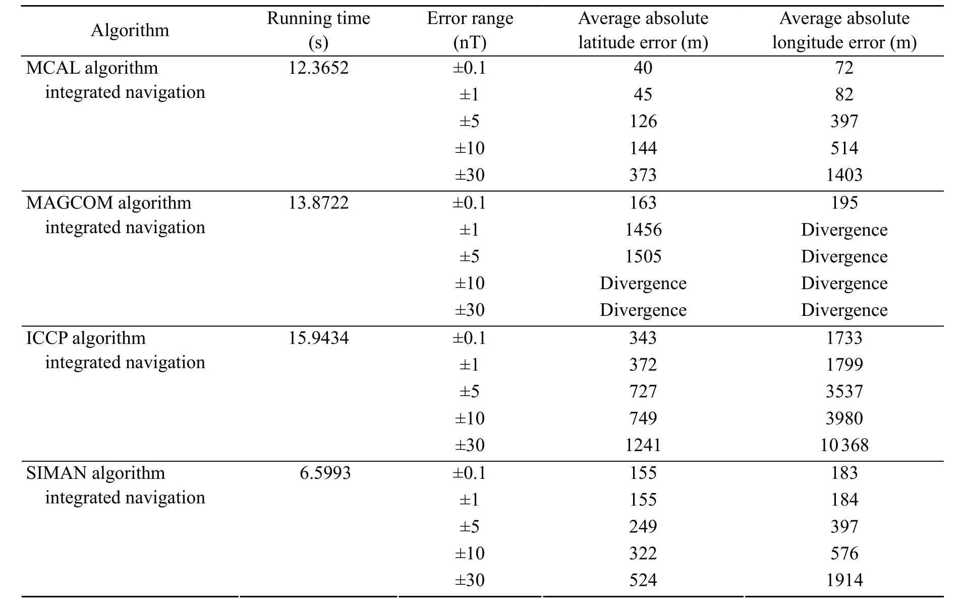
Table 2 Average absolute error when inertial/geomagnetic integrated navigation was used for the period of 420–790 s

The simulation results show that the multigeomagnetic-component assisted integrated navigation system can effectively improve navigation accuracy.In the period of 0–420 s，the positioning error of INS continued to increase.In the period of 420–790 s，with an error range of ±0.1 nT，the multigeomagnetic-component assisted integrated navigation system showed the highest positioning accuracy.The average absolute latitude error was only 40 m，and the average absolute longitude error was 72 m.The navigation range was maintained even when the magnetic error range increased to ±5 nT，and the navigation accuracy was still achieved.When the magnetic error range increased to ±10 nT，the error fluctuated significantly;nevertheless，there was still convergence.The average absolute latitude error was 144 m，and the average absolute longitude error was 514 m.When the random error range is ±30 nT，the average absolute latitude error and longitude error of the MCAL algorithm are 151 m and 511 m lower，respectively，than those of the SIMAN algorithm.The MAGCOM algorithm integrated navigation system had low navigation accuracy;when the magnetic error range was within ±0.1 nT，the average absolute latitude error was 163 m，and the average absolute longitude error was 195 m.Moreover，the error range significantly affected the navigation stability.When the magnetic error range increased to ±1 nT，mismatch occurred，causing non-convergence of the system output.The error of the ICCP algorithm integrated navigation system was significant，and the algorithm took a relatively long time to run.The SIMAN algorithm is a single-point filtering algorithm，and showed the fastest performance.However，its positioning accuracy was slightly lower than that of the proposed algorithm.Note that，for hypersonic vehicles with high Mach numbers，the calculation time is an important factor affecting navigation accuracy.Hence，a more powerful computing platform may be required for the MCAL algorithm.At this point，the SIMAN algorithm is advantageous because of its short computation time.

5 Conclusions

To overcome the mismatch issue of near-space hypersonic vehicles in geomagnetic navigation，where only the information of the main geomagnetic field can be used，we developed the MCAL algorithm.Through the analysis and calculation of the intersection of multiple geomagnetic component isopleths，the real time position of a carrier was estimated.Compared with conventional sequential matching algorithms，this method can provide higher positioning accuracy in the main geomagnetic field environment where near-space hypersonic vehicles are flown.Moreover，it can maintain satisfactory positioning accuracy and stability even when the mixed error increases.

For better results，some improvements are required.First，we did not describe the error model of the main geomagnetic field.The error model is an essential part of the actual geomagnetic navigation application.Second，each time the position is estimated，the algorithm calculates at least two isopleths of the geomagnetic components in the matching area.Although this offers satisfactory positioning accuracy and stability，it requires a strong computing platform.Third，in the case of large errors，the output of the navigation system shows high frequency behavior;hence，the input fed back to the control system may require further processing.

Contributors

Kai CHEN designed the research and provided the funding support.Wen-chao LIANG wrote the first draft of the manuscript and conducted the literature review.Cheng-zhi ZENG processed the data.Rui GUAN revised the final version and developed the software.

Conflict of interest

Kai CHEN，Wen-chao LIANG，Cheng-zhi ZENG，and Rui GUAN declare that they have no conflict of interest.