
Persistence Properties for a New Generalized Two-component Camassa-Holm-type System
2021-05-07 00:58:32YUHaoyangCHONGGezi
工程数学学报 2021年2期
YU Hao-yang CHONG Ge-zi
(1- School of Mathematics, Northwest University, Xi’an 710127;2- Center for Nonlinear Studies, Northwest University, Xi’an 710069)
Abstract: The long time behavior of solutions is one of important problems in the study of partial differential equations. To a great degree, the properties of solutions will depend on those of initial values. The persistence properties imply that the solutions of the equations decay at infinity when the initial data satisfies the condition of decaying at infinity. In this paper,we consider the persistence properties of solutions to the initial value problem for a new generalized two-component Camassa-Holmtype system by using weight functions. Furthermore, we give an optimal decaying estimate.
Keywords: generalized Camassa-Holm-type system; optimal decaying estimate; persistence properties
1 Introduction
In this paper, we consider with the persistence properties of the initial value problem associated with a new generalized two-component Camassa-Holm-type equations[1]
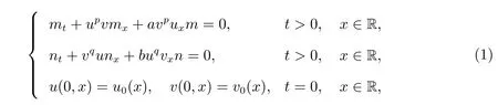
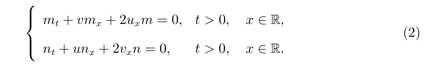
wherem=u−uxx, n=v −vxxandp, q ∈N, a, b ∈R. As shown in[1], this system in(1)has waltzing peakons and wave braking. It is easy to see that ifa=b, p=q, u=v,the system in (1) contains a lot of famous shallow water wave equations, namely, the Camassa-Holm equation (the system in (1) withu=v, p=q= 0, a=b= 2), the Degasperis-Procesi equation (the system in (1) withu=v, p=q= 0, a=b= 3),and the Novikov equation (the system in (1) withu=v, p=q= 1, a=b= 3).On the other hand, one can see that the system in (1) includes the two-component cross-coupled Camassa-Holm equations and Novikov system.
Takingp=q= 0, a=b= 2 in the system in (1), we find the cross-coupled Camassa-Holm equations
Forp=q= 1, a=b= 3, the system in (1) becomes the two-component Novikov equations
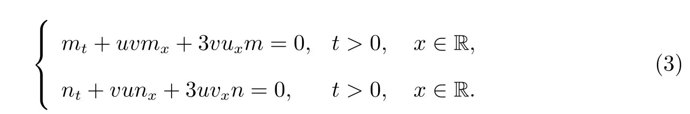
System (2) admits waltzing peakon solutions, but it is not in the two-component Camassa-Holm equations integrable hierarchy[2]. The global existence, blow up phenomenon and persistence properties of the system were discussed in [3,4]. The local well-posedness for the system (3) was established in a range of Besov spaces[5]and in the critical Besov spaces. The results of the persistence properties for the Camassa-Holm equation,the Degasperis-Procesi equation and the Novikov equation can be found in [6–8].
In this paper,we consider the persistence properties of solutions to the initial value problem (1). The solutions of this problem (1) decay at infinity in the spatial variable provided that the initial data satisfies the condition of decaying at infinity. Because all spaces of functions are over R, for simplicity, we drop R in our notation of function space if there is no ambiguity. Before presenting our main results, let us first present the following well-posedness theorem given in [1].
Firstly, we introduce the following spaces[1]
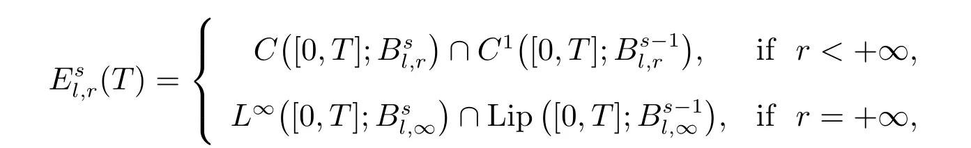
withT>0, s ∈R and 1≤l, r ≤∞.
Lemma 1[1]Assume that 1≤ l,r ≤+∞ands> max{2+1/l,5/2}, let(u0,v0)×. There exists a timeT> 0, and a unique solution (u,v)(T)×(T) to the problem (1). Moreover, the mapping (u0,v0)(u,v) is continuous from a neighborhood of (u0,v0) in×into

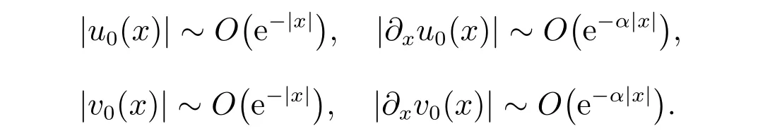
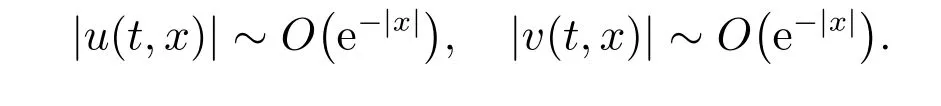
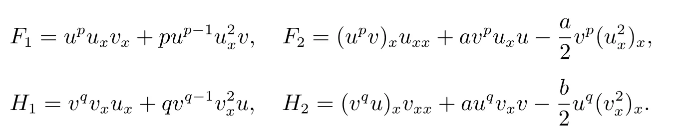
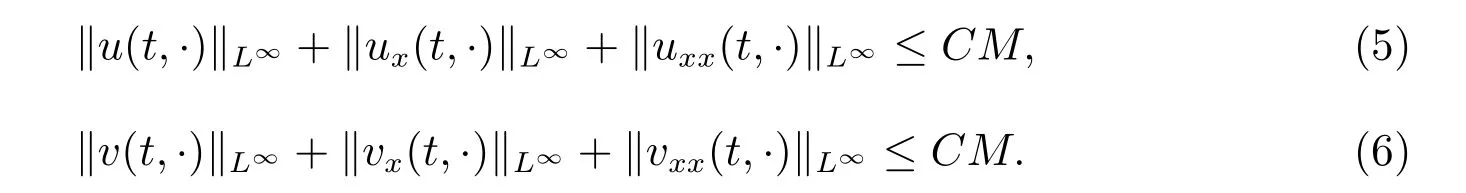
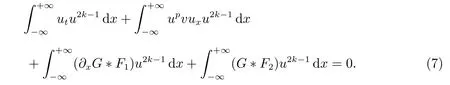
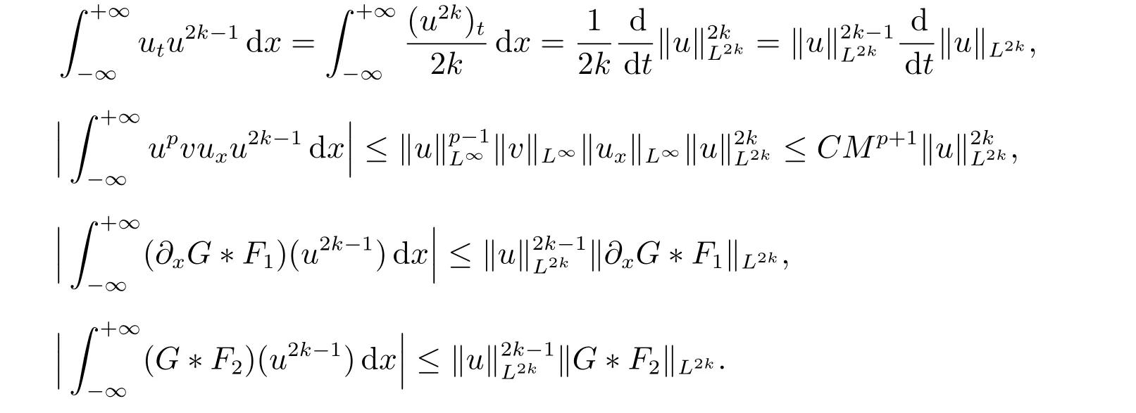
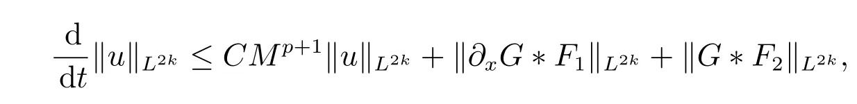
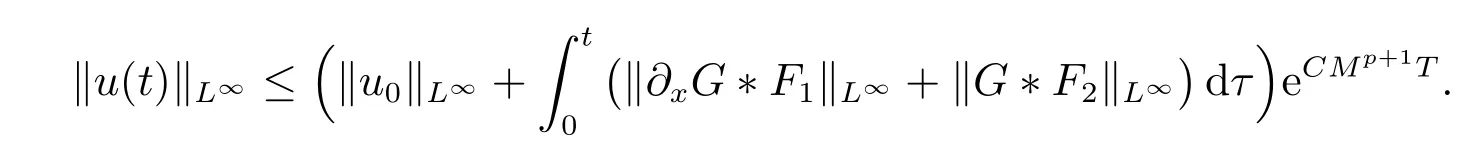
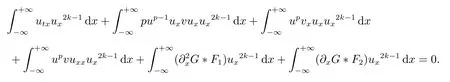
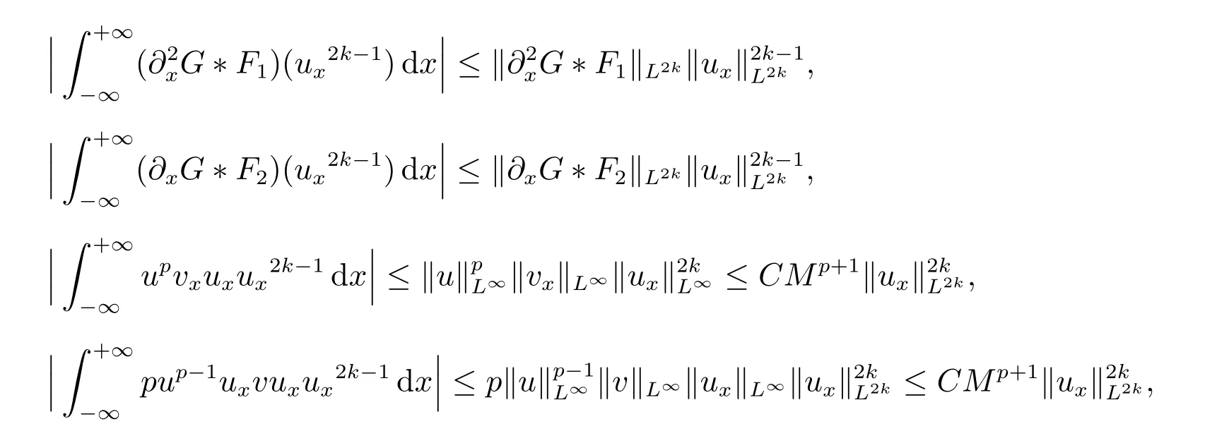
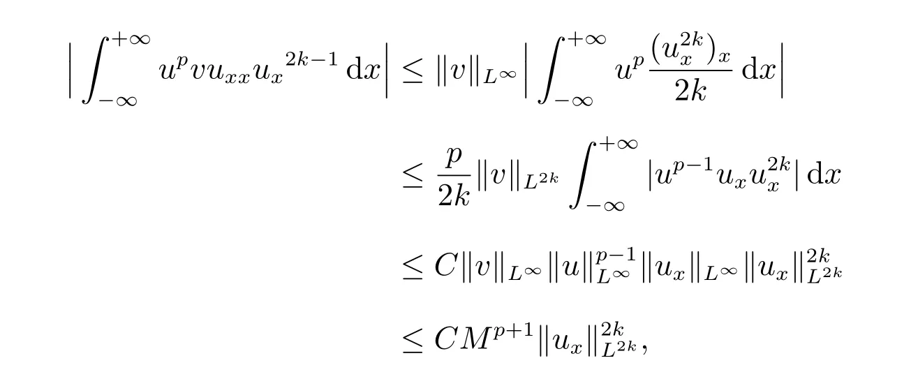
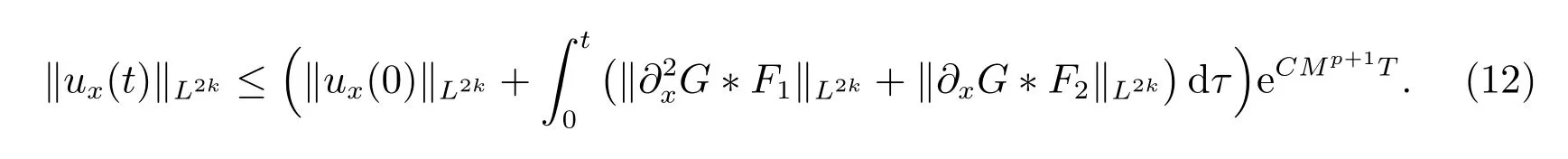
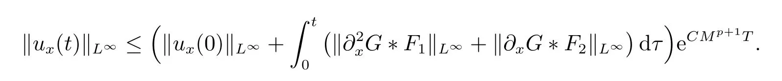
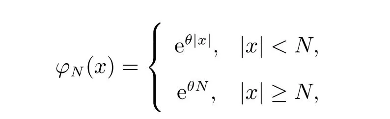
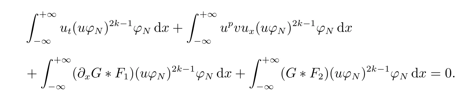
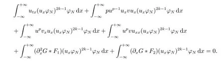
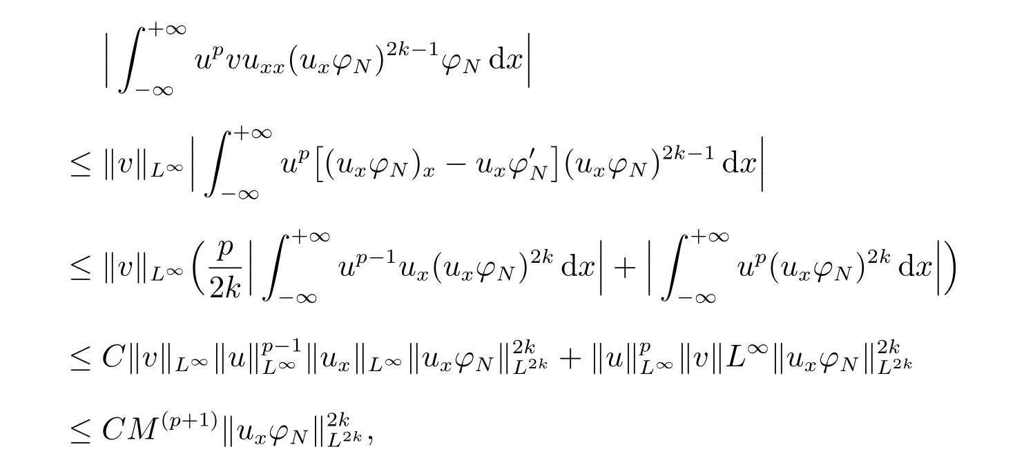
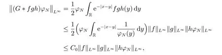
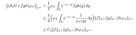
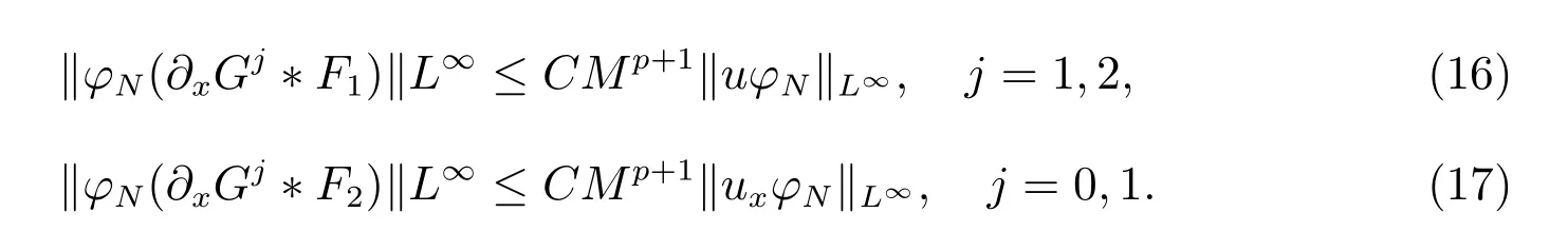
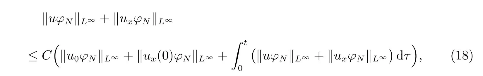
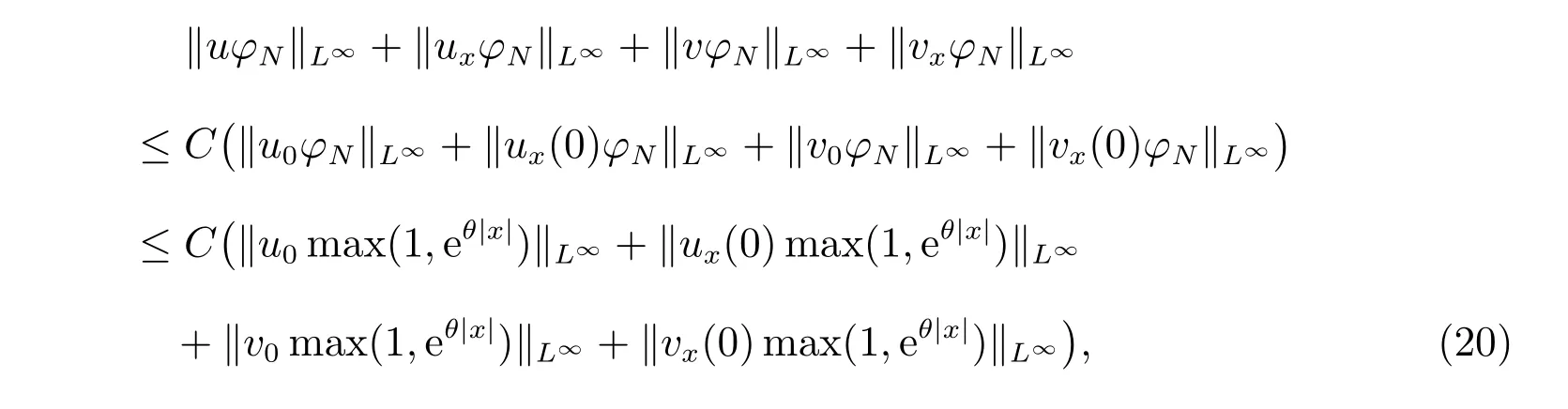
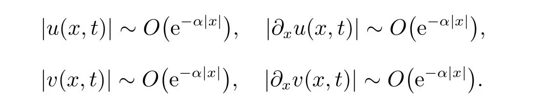
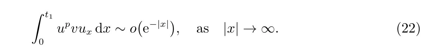
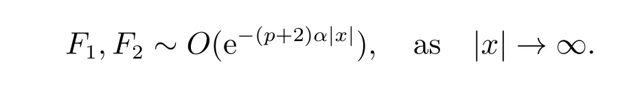
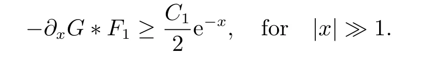
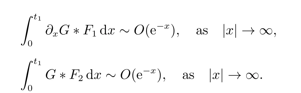
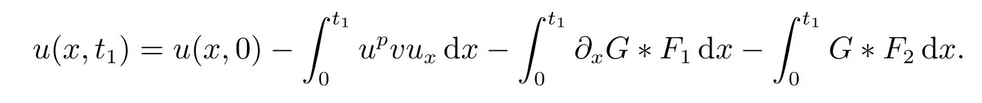
for everys′ Remark 1[1]Thanks toBs2,2=Hs, by takingl=r=2 in Lemma 1 one can get the local well-posedness of the problem (1) in C([0,T];Hs)∩C1([0,T];Hs−1)×C([0,T];Hs)∩C1([0,T];Hs−1) withs>5/2. We may now utilize the well-posedness result to study the persistence properties of the problem(1). We have the following results based on the work for the Camassa-Holm equation[7]. Theorem 1Assume thats> 5/2, T> 0, andz= (u,v)∈C([0,T];Hs)×C([0,T];Hs) is a solution of the initial value problem (1). If the initial datez0(x) =(u0,v0) = (u(x,0),v(x,0)) decays at infinity, more precisely, if there exists someθ ∈(0,1) such that as|x|→∞, Then as|x|→∞, we have Theorem 1 tells us that the solutions of the problem (1) decay at infinity in the spatial variable when the initial data satisfies the condition of decaying at infinity. It is natural to ask the question of whether the decay is optimal. The next result tells us some information. Theorem 2Assume that for someT>0 ands>5/2, Then as|x|→∞, Note thatG(x)=e−|x|is the kernel of the operator(1−∂x2)−1,then(1−∂x2)−1f=G∗f,for allf ∈L2(R).G∗m=uandG∗n=v. The problem(1)can be reformulated as follows where Assume thatz ∈C([0,T];Hs)×C([0,T];Hs) is a solution of the initial value problem(1) withs>5/2. Let hence by Sobolev imbedding theorem, we have Multiplying the first equation of the problem (4) byu2k−1withk ∈N and integrating the result in thex-variable, we obtain (5), (6) and H¨older’s inequality lead us to achieve the following estimates From (7) and the above estimates, we get and therefore, by Gronwall’s inequality For any functionf ∈L1(R)∩L∞(R), SinceF1,F2∈L1∩L∞andG ∈W1,1, we know that∂xG∗F1, G∗F2∈L1∩L∞. Thus,by taking the limit of (8) ask →∞, we get Next, differentiating the first equation of the problem (4) in thex-variable produces the equation Multiplying (10) by (ux)2k−1withk ∈N and integrating the result in thex-variable,we obtain This leads us to obtain the following estimates and using integration by parts we achieve the following differential inequality by Gronwall’s inequality, (11) implies the following estimate Since=G −δ, we can use (9) and pass to the limit in (12) to obtain We shall now repeat the above argument using the weight whereN ∈N andθ ∈(0,1). Observe that for allNwe have Multiplying the first equation of the problem (4) by (uφN)2k−1φNwithk ∈N and integrating the result in thex-variable, we obtain Multiplying (10) by (uxφN)2k−1φNwithk ∈N and integrating the result in thexvariable, we obtain Using integration by parts we get By adding (13) and (14), we have A simple calculation shows that forθ ∈(0,1), For any functionf, g, h ∈L∞, we have and Since∂2xG ∗f=G ∗f −f, Thus, inserting (16) and (17) into (15) we obtain whereCis a constant depending onC0,M, andT. Multiplying the second equation of the problem (4) by (vφN)2k−1φNwithk ∈N and integrating the result in thex-variable, then differentiating the second equation of the problem (4) with respect to the spacial variablex, multiplying by (vxφN)2k−1φNand integrating the result in thex-variable, using the similar steps above, we get Adding (18) and (19) up, we have Hence, for anyN ∈N and anyt ∈[0,T], by Gronwall’s inequality, we get which completes the proof of Theorem 1. Integrating the first equation of the problem (4) over the time interval [0,t1], we get In view of the assumption, we get as|x|→∞, So we obtain and so For we get Moreover Thus Form (23), it follows that Hence Thus, we have Form (21), we get fort1∈[0,T], Then Using the similar steps above, we also get Then as|x|→∞,|v(x,t)|∼O(e−x), which completes the proof of Theorem 2.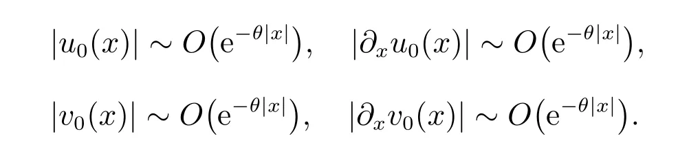


2 The proof of Theorem 1


3 The proof of Theorem 2


- 工程数学学报的其它文章
- Some Properties on the b-chromatic Number of Special Graphs
- Partial Monotonicities of Extropy and Cumulative Residual Entropy Measure of Uncertainty
- Digital Power Exchange Option Pricing under Jump-diffusion Model
- 严格对角占优M-矩阵的逆矩阵的无穷大范数的上界估计
- 二阶混合有限体积法求解Navier-Stokes 方程的稳定性及误差估计
- 一类具有两阶段结构同类相食模型的动力学分析