Stabilization mechanisms of lifted flames in a supersonic stepped-wall jet combustor*

Jin-cheng ZHANG, Ming-bo SUN, Zhen-guo WANG, Hong-bo WANG, Chao-yang LIU

Stabilization mechanisms of lifted flames in a supersonic stepped-wall jet combustor*

Jin-cheng ZHANG†, Ming-bo SUN, Zhen-guo WANG, Hong-bo WANG, Chao-yang LIU

†E-mail: zhangjincheng_512@163.com

Flame stabilization is the key to extending scramjets to hypersonic speeds; accordingly, this topic has attracted much attention in theoretical research and engineering design. This study performed large eddy simulations (LESs) of lifted hydrogen jet combustion in a stepped-wall combustor, focusing on the flame stabilization mechanisms, especially for the autoignition effect. An assumed probability density function (PDF) approach was used to close the subgrid chemical reaction source. The reliability of the solver was confirmed by comparing the LES results with experimental data and published simulated results. The hydrogen jet and the incoming stream were first mixed by entraining large-scale vortices in the shear layer, and stable combustion in the near-wall region was achieved downstream of the flame induction region. The autoignition cascade is a transition of fuel-rich flame to stoichiometric ratio flame that plays a role in forming the flame base, which subsequently causes downstream flame stabilization. Three cases with different jet total temperatures are compared, and the results show that the increase in the total temperature reduces the lift-off distance of the flame. In the highest total temperature case, an excessively large scalar dissipation rate inhibits the autoignition cascade, resulting in a fuel-rich low-temperature flame.

Large eddy simulation (LES); Autoignition; Lifted flame; Flame stabilization; Assumed probability density function (PDF)

1 Introduction

Although hypersonic vehicles powered by scramjet engines have developed rapidly, they continue to face challenges with regard to stable and highly efficient combustion. Complex physical- chemical phenomena, such as mixing, ignition, flame propagation, and stabilization, are not yet fully understood (Clark and Bade Shrestha, 2013), especially for scramjets operating at high flight Mach numbers, where autoignition is more common. The purpose of this paper is to study combustion characteristics in hypersonic conditions involving autoignition and flame, thus providing a theoretical basis for combustor optimization.

The stabilization mechanism of lifting flames is currently viewed in three ways: the premixed flame model, the large eddy model, and the extinction model (Lawn, 2009; Karami et al., 2015). In the premixed flame model, the flame base is considered to be premixed, and the flame can be stabilized when the local flame velocity and flow velocity are balanced (Chung, 2007). The large eddy theory points out that the large eddies on the boundary of the jet will cause the hot products and air to be re-blended with the rich mixture to form flammable pockets (Miake- Lye and Hammer, 1989). The extinction model takes into account the effect of the scalar dissipation rate. It is believed that the scalar dissipation rate determines the lifted height and the flame is stable near the critical scalar dissipation rate (Watson et al., 2003). These theories are widely used in environments with low-temperature oxidants. However, when the oxidant is heated, autoignition generally occurs and a different flame stabilization mechanism is observed.

Many experiments and numerical studies have reported observations of a lifted flame dominated by autoignition in different configurations. For studies of turbulent flames in combustors, coaxial jets with simple structures are often used as models. In the coaxial jet experiments performed by Cheng et al. (1991), a flame generated by hydrogen and oxygen reactions existed at a certain distance downstream from the jet outlet. They defined and calculated Damköhler numbers, which showed that the finite rate of the chemical reaction was an inherent cause of flame lift and stabilization. Cheng et al. (1991) also found that the three-body reaction inhibited heat release downstream. Boivin et al. (2012) presented a simulation of coaxial jet combustion using a three- step simplified reaction mechanism of hydrogen and oxygen, in which an autoignition identification method based on chemical explosive mode analysis (CEMA) was applied. The outcome showed that the upstream “finger-like” autoignition region was the initial reaction stage. Moule et al. (2014) carried out a numerical simulation based on Cheng et al. (1991)’s experiment. They pointed out that the autoignition effect and compressibility effect jointly control the chemical reaction process. The autoignition process started chain reactions which generated water. A high-temperature reaction zone after the shock wave dominated the release of heat; thus, the lifted flame stabilized. Bouheraoua et al. (2017) concentrated on shocks and ignition, and concluded that transient bow shock induced by heat release leads to flame oscillation.

In a real combustion chamber, there are more complex boundary conditions that should be considered. A supersonic combustor with a step—a configuration that is close to that of a real combustion chamber—is often used to study turbulent flame organization. The stepped-wall jet combustor has similar structures to a supersonic mixing layer. Moreover, the development of the wall boundary layer affects the turbulent mixing layer and the heat release of the chemical reaction, and vice versa. Burrows and Kurkov (1973) experimented with the mixing of inert gases and combustion of vitiated air. The data showed that the reaction thickened the mixing layer, and the flame lift-off distance matched the inlet velocity and hydrogen ignition delay time. The total temperature, total pressure, and component distribution data obtained during the experiment became the basis of later numerical studies. Based on Burrows-Kurkov’s experiment, Engblom et al. (2005) verified the performance of the Wind-US method and discussed the sensitivity of the autoignition location to the turbulence model and Prandtl number. Edwards et al. (2012) described large-eddy/Reynolds-averaged Navier-Stokes simulations (LES/RANS) of this experiment. Resulting from simulations of different boundary conditions and reaction mechanisms, Engblom et al. (2005) indicated that the flame exhibits a transition from a partially premixed flame to a diffusion flame. Vyasaprasath et al. (2015) presented a numerical simulation based on detached eddy simulation (DES), and the results underestimated the maximums of H2O concentration and total temperature in the experimental data. The subgrid-scale (SGS) model and chemical reaction mechanism were considered to be the main causes of this deviation. Few other works have focused on flame stabilization in scramjet engines.

In scramjet combustors, there generally is not sufficient residence time for the mixing process of the fuel and oxidant. However, shear layers formed by jets provide chances and places in which eddies roll and break apart with local deceleration and heating. Autoignition onsets atmr(wheremris the mixture fraction with the most reactive reaction) of the braided areas and develops autoignition kernels for suitable conditions (Mastorakos, 2009). As radicals are transported downstream, chain reactions induce the formation of a turbulent diffusion flame with a certain lift-off distance. In-depth studies and systematic investigations of the stabilization regime dominated by autoignition are rare.

In this study, we performed LESs based on the configuration of Burrows-Kurkov’s experiment (Burrows and Kurkov, 1973). First, the solver and models were validated by comparing the numerical results with the experimental data. Then, the experiment- based simulation was analyzed in detail to reveal the flame stabilization mechanisms. Furthermore, two additional jets with different total temperatures were also simulated to study the influence of jet total temperature on combustion characteristics.

2 Models and methods

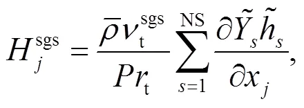
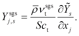
With the development of computer technology, LESs are widely used in research because they have a greater ability to obtain accurate results for turbulent reacting flow than the RANS (Pitsch et al., 2008); additionally, LESs are more consistent with experiments in many complex problems. For supersonic compressible flows, an LES solves the Navier-Stokes (N-S) equations obtained by spatial filtering and Favre averaging (Garnier et al., 2009):

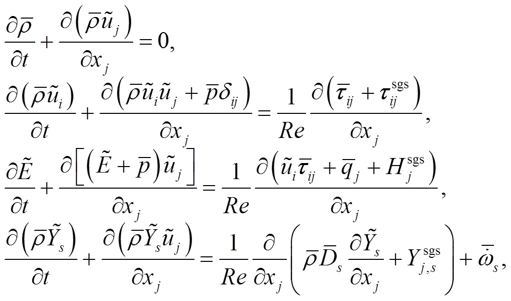
The filtered viscous stress tensor is related tosgs:

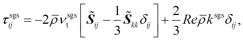
The subgrid turbulent kinetic energy denotes the interaction of large- and small-scale vortices, which needs further treatment. Moreover, a filtered chemical reaction source term must be closed considering the turbulence effect. The turbulence model for closingsgsand the turbulent combustion model for closing the component source term are described below.

2.1 Turbulence model

In the current work, turbulence is modeled by the equation model proposed by Yoshizawa and Horiuti (1985):

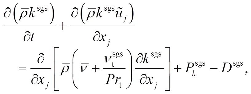
The constants (t,t,, andd) used in the above model refer to our previous work (Wang et al., 2014; Liu et al., 2016, 2017).

2.2 Combustion model

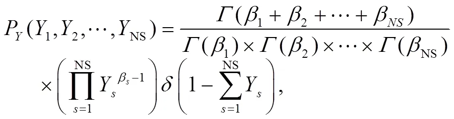
The assumed probability density function (PDF) method borrows ideas from the transport PDF and removes the limitation of computational burden on the bulky transport PDF method (O’brien, 1980). A finite amount of moment information is introduced to construct the PDFs of temperature and composition; thus, the unclosed chemical reaction source terms are obtained in the form of mean scalars and turbulence scalars.

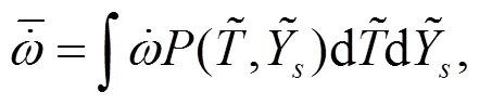
Some studies have shown that the PDF model is not sensitive to the form of function(Frankel et al., 1990; Baurle et al., 1995). The function type can be set in advance, which is also a superiority of the assumed PDF. In this way, solving the probability density transport equation by the Monte Carlo method can be avoided to save computational cost. The specific form of Eq. (6)is given below:

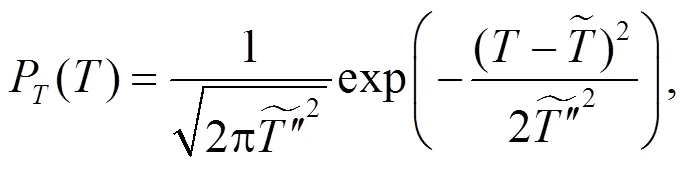
Assume that temperature, composition, and density are independent of each other:

The Gaussian distribution of the temperature and the multivariatedistribution of the components were used in cavity jet combustion by Wang et al. (2013), and the simulation results were in agreement with the experimental results. The current study also selects such a combination of functions to employ the assumed PDF. The reaction mechanism used in the assumed PDF is the Jachimowski mechanism (Jachimowski, 1988). The specific process is not repeated, as this information is described in detail in (Wang et al., 2011).

For the approach combining the assumed PDF and RANS, the suitability of the assumed PDF has been certified for simulating supersonic reacting flow, especially when the variance information is already known (Förster and Sattelmayer, 2008). The LES provides a more detailed description of turbulence and is a more attractive solver for reacting flow. Some studies have successfully coupled assumed PDF with LES (Liu et al., 2019). In this study, the effectiveness of this method for turbulent flame problems is verified, and the autoignition and flame stabilization problems are analyzed in depth.

2.3 Numerical schemes

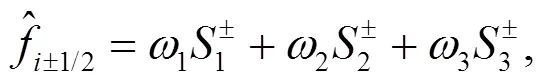
Specific forms and coefficients of the combination can be found in (Sun et al., 2008).

A very efficient time advancement scheme, which is popular in supersonic unsteady flow, is a dual time-step approach (Jameson, 1991). As an implicit method, a dual time step requires an iterative algorithm to solve semi-discretization equations. Lower-upper symmetric Gauss-Seidel (LU-SGS) (Yoon and Jameson, 1988) was selected for the current LES simulations, and the convergence criterion is presented in (Wang et al., 2010). The WENO matched with LU-SGS is a mature, reliable solution of computational fluid dynamics (CFD), which performs robustly with high precision and efficiency.

3 Validation

Before further analysis, the models and methods must be validated. The computational settings used in the study are introduced, and a comparative analysis of the simulated results and experimental data processes is performed.

3.1 Computational grids and conditions

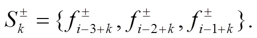
The schematic of the computational domain consisting of Burrows and Kurkov (1973)’s experiments is shown in Fig. 1. This study utilized a 2D-RANS for the turbulent plate boundary layer in advance to confirm the minimum cell spacing at solid surfaces. The results provided 3D-LES with a turbulent inlet including the boundary layer. By intercepting the profile 427.88 mm downstream of the 2D-RANS inlet, a 10-mm boundary layer (Edwards et al., 2012) is acquired, which is applied to the inflow boundary of the 3D-LES. Then, 3D-LES is implemented in the 560-mm-long region that has a 4.76-mm-high downward step (containing a 0.76-mm-high lip) located 160 mm downstream, where the H2jet enters. The upper border with the reflection boundary remains horizontal, whereas the lower wall surface exhibits a slight expansion. To minimize the computational cost, the width is only 10 mm, and both the left and the right sides are periodic boundaries.

Abundant eddies form in the jet shear zone, which is a significant location, and the other hotspot is the area near the solid nonslip wall where boundary layers are generated. The grid should be clustered in the above regions to meet the mesh resolution demands of LES. Grid points within the boundary layer are refined to ensure that the height of the first-layer grid satisfies+=1. According to 2D-RANS, the height was set to 0.0075 mm. Moreover, for the purpose of suppressing numerical oscillations, a buffer zone is installed next to the exit, and the mesh in this zone needs to be gradually stretched. In this study, we designed three kinds of meshes with different degrees of refinement designed for mesh independence verification. Mesh distribution of grid-2 in the-centerplane near the step is shown in Fig. 2. Exhaustive mesh information is listed in Table 1.

The jet and inflow conditions applied at both the 2D-RANS plate and the 3D-LES combustor are listed in Table 2.

3.2 Validation comparisons with available data

The experimental data from Burrows and Kurkov (1973) supports the validation of the present code and mesh. The total temperature is a crucial parameter in the reacting flow field, which is determined by the local static temperature and Mach number. The profiles of the stagnation temperature gained close to the exit of the combustion chamber (=356 mm) are shown in Fig. 3. The numerical results for different grids are given by curves, and the experimental results are marked by squares. A gradual increase in the reaction zone prediction capability from grid-1 to grid-3 can be clearly visualized. The results obtained by grid-2 were close to those obtained by grid-3; hence, the results from LES with grid-2 are considered to be convergent and the following analysis and discussion are based on the results of grid-2.

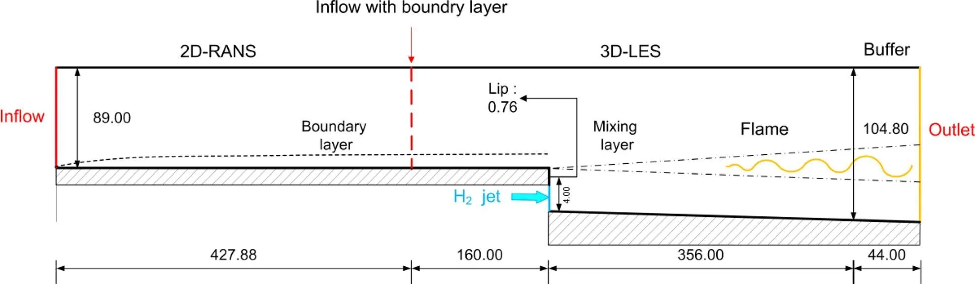
Fig. 1 Schematic of the computational domain (unit: mm)

Table 1 Grid numbers and corresponding resolution

N,N, andNare the numbers of grids in three directions, correspondinglyΔ+,Δ+, andΔ+are the ratios of the grid size in the three directions to the wall distance when+=1

Table 2 Reference conditions for Burrows and Kurkov (1973)’s experiments

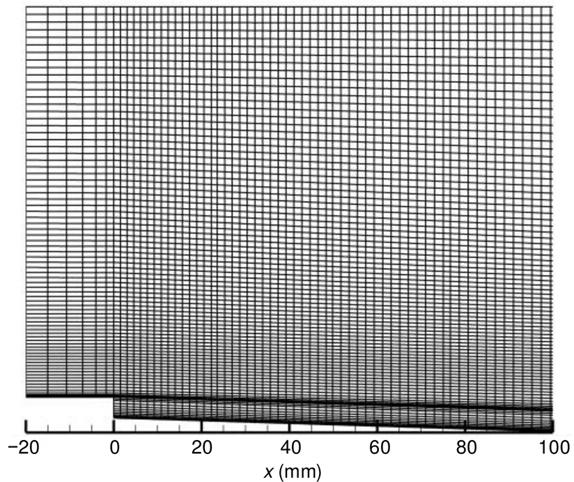
Fig. 2 Mesh distribution of grid-2 in X-Y centerplane near the step

The total temperature increase near the wall was almost completely coincident with the experimental data. This uniformity indicated that the development of the boundary layer was appropriate. Nevertheless, the predicted total temperature at the center of the reaction zone was slightly lower than the experimental data. Component concentrations embodying mixing processes and chemical reactions were similarly extracted for comparison at the exit position in Fig. 4. These four components exhibited the same trends as those observed in the experiment, whereas the peak value of the calculated mole fraction of H2O was lower than that in the experiment. Meanwhile Figs. 3 and 4 show the result obtained by Edwardset al. (2012), which also underestimated the peak stagnation temperature and was close to our results. In the near-wall area, we obtained more similar results to the experiment, but the prediction of the thickness of the reaction zone was relatively poor.

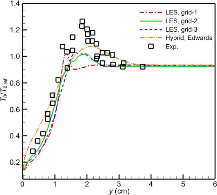
Fig. 3 Stagnation temperature profiles at the combustor exit (x=356 mm)

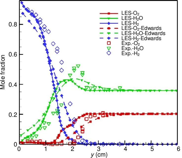
Fig. 4 Mole fraction profiles at the combustor exit (x=356 mm)

The differences in the total temperature and component peak may be due to the following reasons. First, boundary conditions can often determine the accuracy of calculation results (Star et al., 2006). In the experiment, the heat transfer process on the wall of the combustion chamber was very complicated, and it was difficult to accurately formulate such boundary conditions in numerical calculations. Moreover, the simulation in this paper was limited by the amount of calculation; therefore, we did not consider the effect of limited space. The side of the combustion chamber used periodic boundary conditions instead of solid walls. In addition, the deviation was likely to be affected by the reaction mechanism. The intensity of the reaction and the thickness of the flame were underestimated. There may be other reasons, including potential errors in the experimental measurements.

The LES/RANS simulation by Edwards et al. (2012) was in agreement with the experimental data for nonreactive mixing of a hydrogen jet. For vitiated-air mixing and combustion, defects remained at the maximum values of total temperature and mole fraction. Fig. 5 shows the time-averaged contours of static temperature at the-centerplane. The basic structure of the combustion field, the lifted height of flame, and the shape of the reaction zone obtained in this study are all consistent with Edwards et al. (2012). It is a further conclusive evidence for the reliability of the present LES solver.

In summary, the simulated results in this paper are credible; furthermore, they support the following discussions.

4 Results and discussion

There are intricate coupling effects between flow and combustion in the flow field; consequently, flame stabilization is determined by many factors. This section first describes the basic characteristics of the flow field and then analyzes the flame stabilization mechanism and explains the effect of autoignition. Next, simulations of the different total temperatures of jets are compared, and the effect of the total temperature on the reacting flow field is summarized to deepen understanding of the stabilization mechanism.

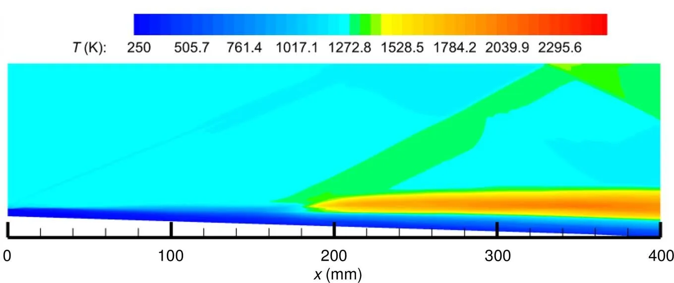
Fig. 5 Time-averaged temperature contours at the X-Y centerplane

4.1 Flame stabilization mechanism of reacting flow fields

In the reacting flow field, large-scale mixing is controlled by the shear vortex, whereas small-scale mixing is controlled by turbulent fluctuations, which significantly affects the occurrence of chemical reactions and flame stabilization. For scalar mixing characterization, the definition of the mixture fraction is introduced:

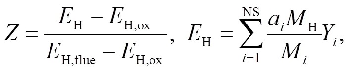
whereHis the mass fraction of hydrogen,H,oxandH,flueare the mass fractions of hydrogen in the oxidant and in the flue, respectively.a,M, andHrepresent the number of hydrogen atoms in theth species, the molar mass of hydrogen atoms, and the molar mass of this species, respectively. Such a definition gives the mixture fraction a normalized characteristic:min=0 represents the incoming oxidant side,max=1 is the fuel side, and whenis between 0 and 1, it can characterize different local equivalent ratios.

Fig. 6 shows the dimensionless density gradients (Ñ/∞, whereÑis the density gradient and∞is the density of the inflow from inlet) of the-central section of the mixing case and the reacting case. The red line is the contour of the mixture fraction=0.1. The density gradient indicates the wave and vortex structure, and the mixture fraction is used to describe the fuel blending. Outside of the boundary layer, a series of expansion waves at the jet inlet and shear layer are also marked as black, which signifies that the density changes drastically in both the pure mixing and the reacting cases. The difference was that an additional shock wave appeared downstream in the combustion flow field in the reacting case. The process of flow structure formation can be inferred from this situation: the incoming stream contacts the jet at the inlet and expands mildly; because of Kelvin-Helmholtz instability, mixing is accompanied by vortex shearing and rolling up. In the reacting case, a shock wave located at about=200 mm was induced by heat release, which had a substantial production rate in this location. The other phenomenon that demonstrated the influence of combustion on the flow regime was the lift of the shear layer after the shock wave. Compared with the top image, the outer contour of the shear layer downstream of the bottom image is clearly separated from the isoline=0.1, indicating that the shear layer became thicker after the shock.

Snapshots of the dimensionless temperature (/∞, where∞is the temperature of inflow from the inlet) are shown in Fig. 7, in which Fig. 7a shows the temperature distribution that was only dominated by mixing and Fig. 7b shows the effect of combustion supplemented by reaction. When<100 mm, the reacting case manifested similar to mixing, and there were only sporadic areas preheated by high-enthalpy flow. Then, when 100 mm<<200 mm, finger-shaped high-temperature zones appeared, which were embedded between vortices. Further downstream, when>200 mm, the high-temperature area was connected into one piece and floated on the low-temperature jet. The same segmentation phenomenon also appeared in the OH radical snapshot, as shown in Fig. 8. There was essentially no OH generation before=100 mm, whereas an evident mass fraction of OH appeared after>150 mm. The solid black line in Fig. 8 is the contour of the stoichiometric ratiost=0.0312. OH radicals spread on both sides of the contour line, and the closer the distance to the line, the greater the mass fraction. This means that lean and rich reactions coexisted; the specific spatial distribution characteristics will be illustrated in detail below. Looking at Figs. 7 and 8, the flow field after the jet inlet can be divided into three regions: mixing zone (<100 mm), autoignition induction zone (100 mm<<200 mm), and flame zone (>200 mm).

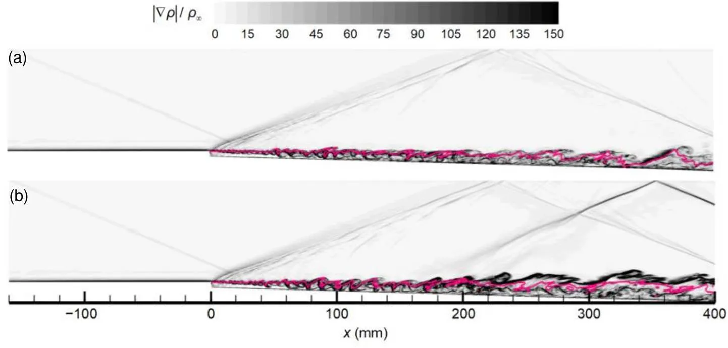
Fig. 6 Density gradients of the X-Y centerplane of the mixing case (a) and the reacting case (b)

The red line is the contour of the mixture fraction=0.1. References to color refer to the online version of this figure

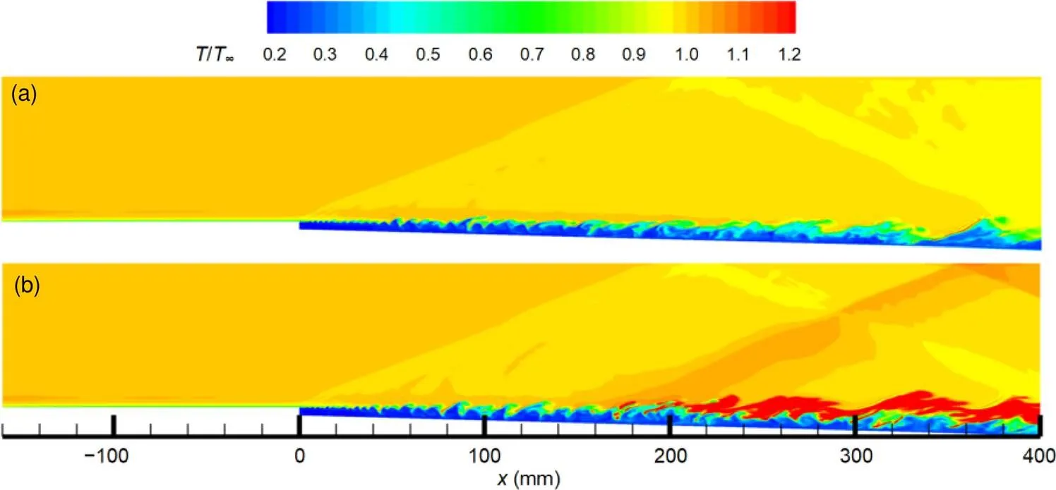
Fig. 7 Temperature of the X-Y centerplane of the mixing case (a) and the reacting case (b)

The flame was finally stabilized near=200 mm due to ignition delay, and the flame may have been partially premixed. To distinguish the diffusion flame from the premixed flame in the flame zone, the following definition of the flame index is used:

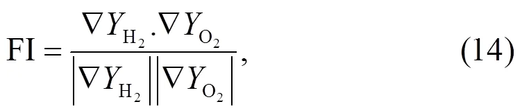
In a diffusion flame, the fuel oxidant gradient is in the same direction (FI>0); in a premixed flame, the opposite is true (FI<0) (Fig. 9). After the flame is lifted, there is a clear layered structure. By counting the probability density distribution of the FI, a typical partial premixed flame structure may be summarized: diffusion flames mainly exist near the stoichiometricof the jet edges, and the density-weighted ratio is 72.20%. The remaining 27.80% are premixed fuel-rich flames closer to the interior of the jet.

As described above, the jet was mixed with the incoming stream stagnated on the upstream wall; autoignition occurred when 100 mm<<200 mm, and then OH radicals were produced while autoignition flame kernels formed. The thermal expansion induced a shock wave, and the flame propagated downstream and stabilized at approximately>200 mm. The flame stabilization mechanism is analyzed below.

Based on the preceding zone partition, data was extracted from three flow direction locations (take=50, 150, and 300 mm as references) in different regions and organized in Fig. 10. These four graphs illustrate variations in the dimensionless velocity/∞and mixture fractionalong the wall distance−walland variations in the dimensionless temperature/∞and OH mass fraction distributions with respect to the mixture fraction. There were two extreme points in the velocity profile of the mixing zone (=50 mm): the maximum point was 14.2% higher than the velocity of the jet inlet (jet), whereas the minimum point was developed from the boundary layer of the incoming wall. These two extreme points in the autoignition area moved closer to the middle. In the downstream flame zone, the extreme point disappeared and the curve became monotonic. At=150 mm, a low-speed interval offered a longer mixing time to autoignition. The solid line with a lower slope reflects a low-velocity gradient circumstance, which is conducive to flame stabilization. Curves ofat different positions show a trend of mixed layers becoming thicker, which reduced the stretch of the flame by the flow.

Figs. 10c and 10d show different chemical reaction characteristics in the three regions. The temperature in the mixing process satisfied the negative correlation with, and no reaction generated OH. In contrast, in the autoignition zone, the temperature was basically unchanged, whereas a small amount of OH was distributed on the fuel-rich side>0.0312. The temperature increased conspicuously in the flame region; furthermore, a peak was located near the stoichiometric fraction. Such features indicate that the reaction entered a steady state and showed diffusion flame characteristics. Spatial distributions of autoignition and flame confirm that autoignition was a key reason for downstream flame stabilization.

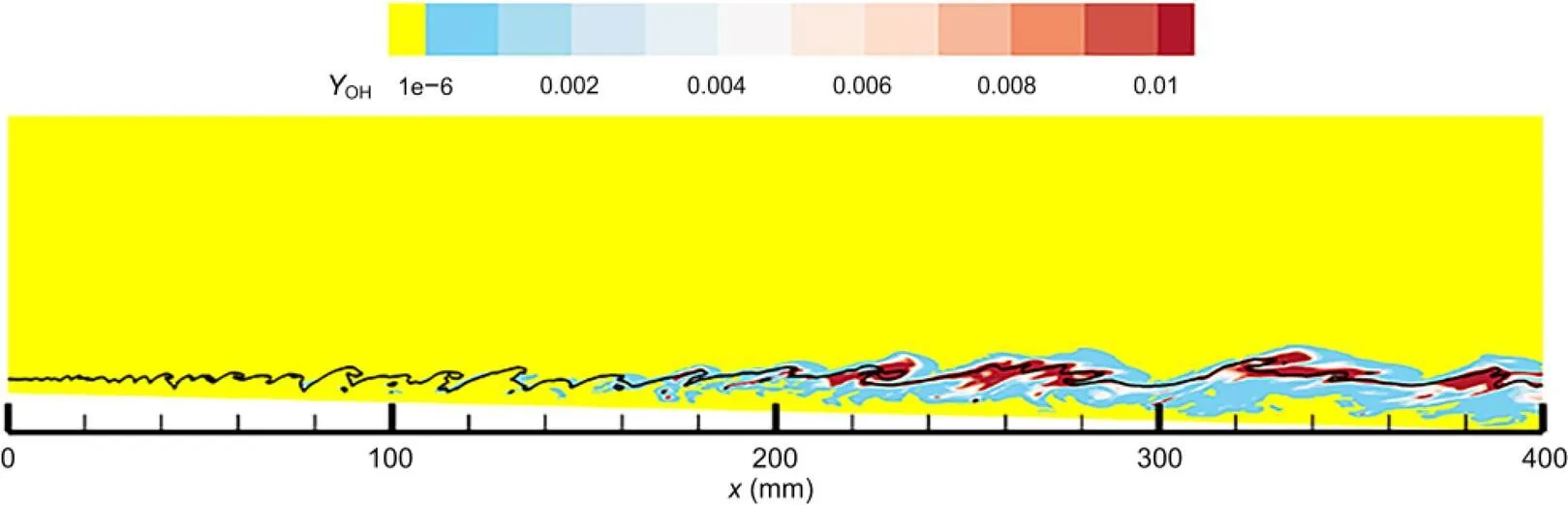
Fig. 8 OH mass fraction contours at the X-Y centerplane

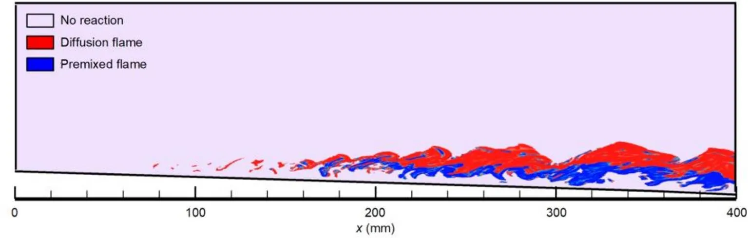
Fig. 9 Contours of flame index

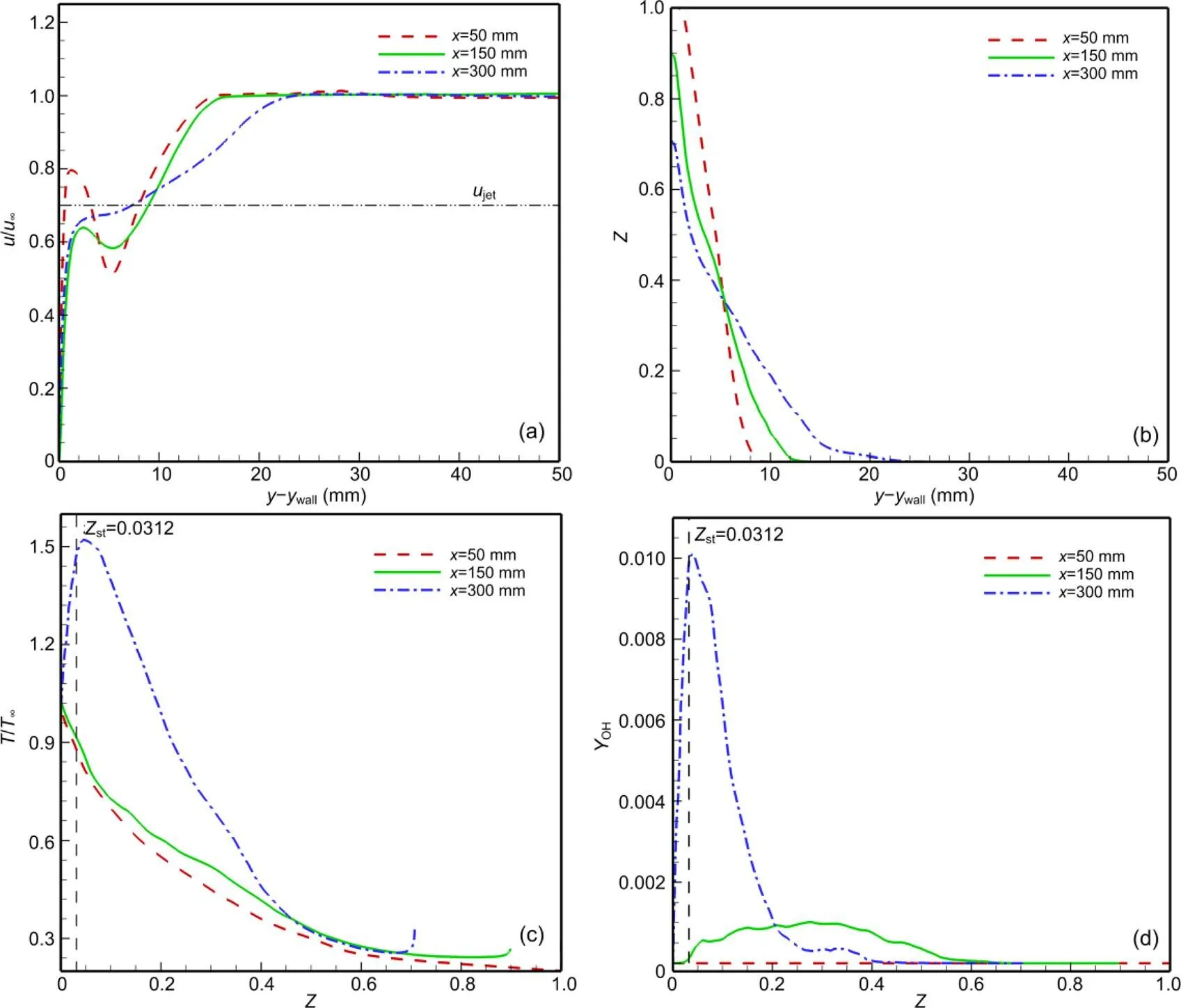
Fig. 10 Velocity (a), mixture fraction (b), temperature (c), and OH mass fraction (d) distributions at three positions (x=50, 150, and 300 mm)

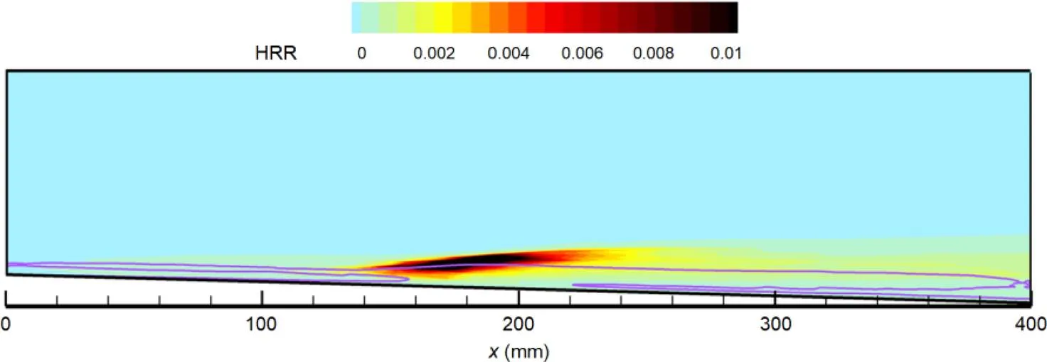
Fig. 11 Contours of heat release rate

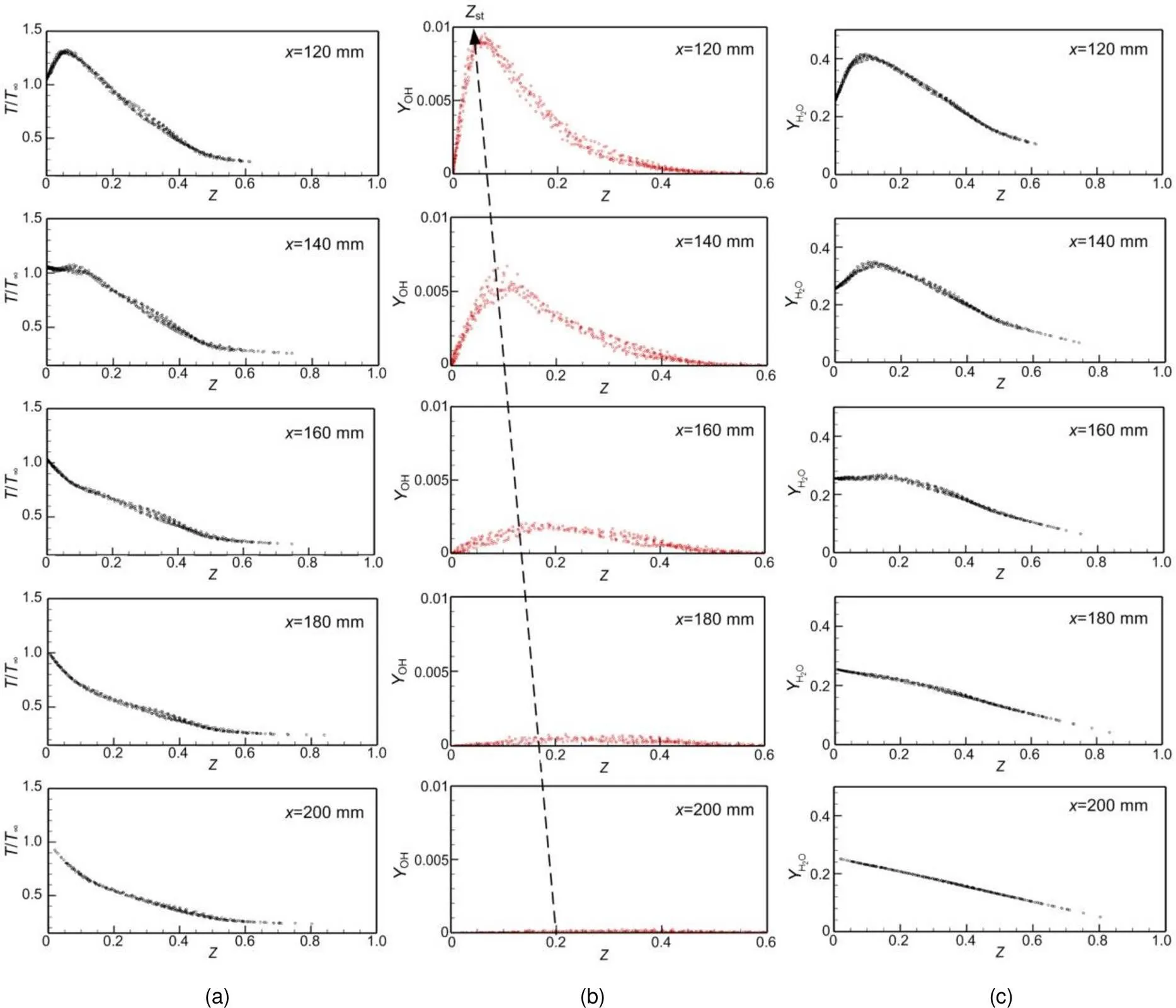
Fig. 12 Scatter plots of temperature (a), OH mass fraction (b), and H2O mass fraction (c) at different distances extracted from x=120 mm to x=200 mm (20-mm increment from top to bottom)

Based on the above analysis, the flame stabilization mechanism of the jet can be summarized as follows: the boundary layer and the shear layer become thicker and merge along with development, and a region of low speed and low shear is generated, which creates very conducive mixing conditions. The ignition cascade continues to provide a flame kernel and diffusion in the vicinity ofstto form a flame accompanied by a large amount of heat release. Thermal choking induces a shock wave that thickens the shear layer and accelerates the reaction behind the shock to promote flame stabilization.

4.2 Influences of jet total temperature

The previous section covered the flame structure and flame stabilization mechanism under experimental conditions. We found that the shock caused by compressibility had an important effect on flame stability, and autoignition was the essential reason for flame stability. In experiments and practical applications, fuels are often preheated before being injected. It is valuable for engineering application to study the effect of total temperature of jet on the reacting flow field. This section shows the simulated results for jets with different total temperatures. By comparing the lift-off height and the parameters of the reacting flow, the flame stabilization mechanism is further revealed, and the influence of the total temperature of the jet on the lifted flame can be summarized. The selected conditions were0,jet=314 K (Case 1),0,jet=625 K (Case 2), and0,jet=900 K (Case 3), where0,jetis the total temperature of jet.

Figs. 13 and 14 show the time-averaged static temperature and the time-averaged mass fraction of OH for Cases 1–3, respectively. It is obvious that the flame lift-off distance decreased with the increase in the total temperature of jet: approximately 180 mm for Case 1, approximately 130 mm for Case 2, and approximately 70 mm for Case 3. The shock position also moved upstream. In Fig. 14, the black line marks a subsonic region near the wall; the higher the jet temperature, the larger the range of this region. The coupling effect of the chemical reaction and compressibility was reconfirmed: the heating and choke caused by heat release in the compressible fluid provided positive feedback which reduced the delay of the chemical reaction and enhanced mixing.

The lift-off distances can generally be estimated from the ignition delay and the jet velocity. Fig. 15 shows the delay times for different temperatures, which were calculated by the Jachimowski mechanism at an initial pressure of 100 kPa) and at the equivalence ratio=1 (=st). The square mark in the figure is the ignition delay time (ig) corresponding to the operating conditions of the three cases. The temperature and speed selected for the predicted lift-off distances are given in Table 3. The predicted delay distances and the lift-off distances given by simulation are also listed. The predicted values were smaller than the average simulated values. These two lift-off distances were consistent, indicating that autoignition was indeed the cause of initial flame formation.

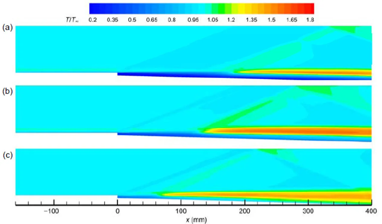
Fig. 13 Time-averaged temperature snapshots for different total temperatures of jet: (a)–(c) Case 1–Case 3

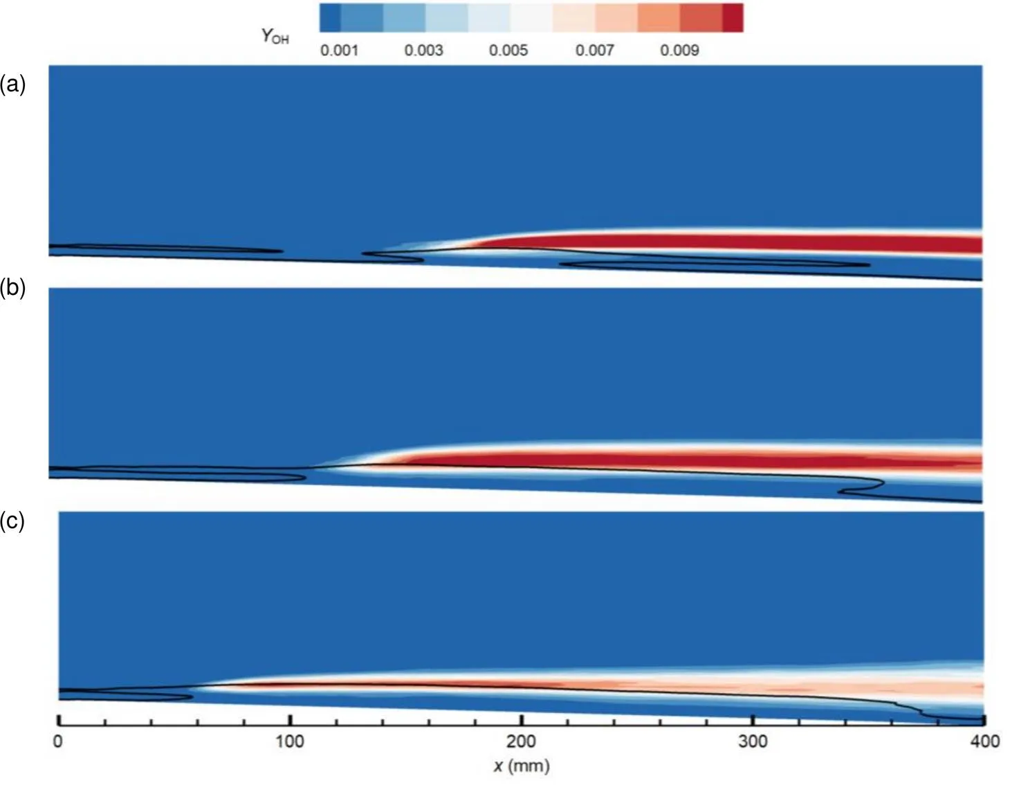
Fig. 14 Time-averaged OH mass fraction snapshots for different total temperatures of jet: (a)–(c) Case 1–Case 3

The total temperature of jet caused macroscopic differences in lift-off distances. In addition, the spatial distribution of chemical reactions needs further discussion. The stoichiometric ratio contour in the average flow field was extracted to analyze the reaction characteristics in the flow direction. Fig. 16 demonstrates the temperature and OH mass ratio on the isoline=st. The three typical zones are arranged in sequence: the mixing zone with no reaction, the autoignition zone, and the flame zone. The temperature response to the chemical reaction was slightly delayed compared to the OH mass fraction response.After the highest temperature in Case 3, when= 200 mm, the OH mass fraction and temperature exhibited a slight downward trend, whereas the other two cases maintained stable values after flame formation.

Fig. 15 Autoignition delay time predicted by the Jachimowski mechanism

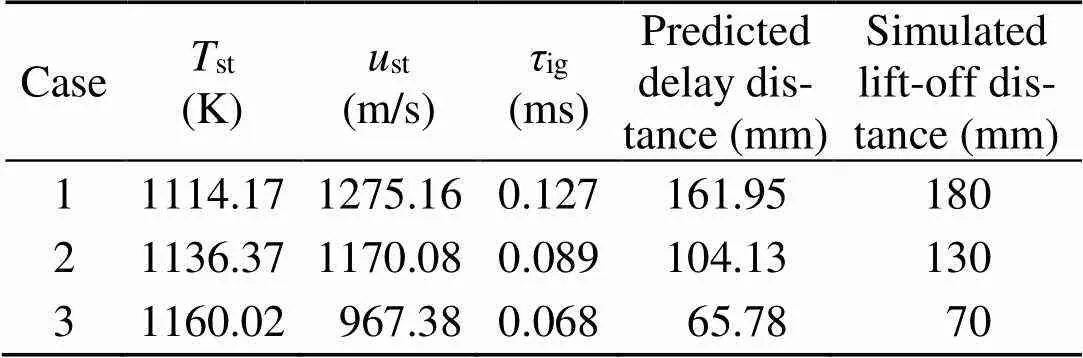
Table 3 Flame lift-off distance predictions

standstmean the temperature and velocity when=st, andigis the ignition delay time

To reveal the flame temperature distribution in Case 3, which was different from that in the other operating conditions, a quasi-1D reaction kinetics analysis was performed at the initial ignition position and the exit position perpendicular to the OH. Fig. 17 shows the quasi-1D distribution of OH and H2O under different conditions and at different locations. Similar fuel-rich and fuel-lean reactions occurred in the autoignition region of the three operating conditions; when diffusing downstream, the OH peak in Case 3 did not appear at the stoichiometric ratio. Hence, there was still a large part of the rich flame in Case 3, preventing achievement of maximum temperature. From the perspective of water generation, the peaks of water all fell on the rich side, indicating that the chain reaction from the generated water consumed hydrogen.

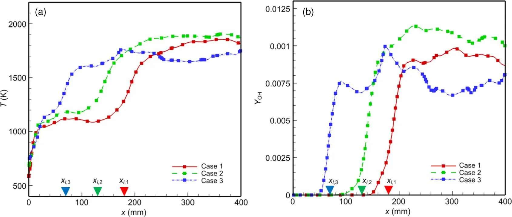
Fig. 16 Variations in temperature (a) and OH mass fraction (b) at Zst

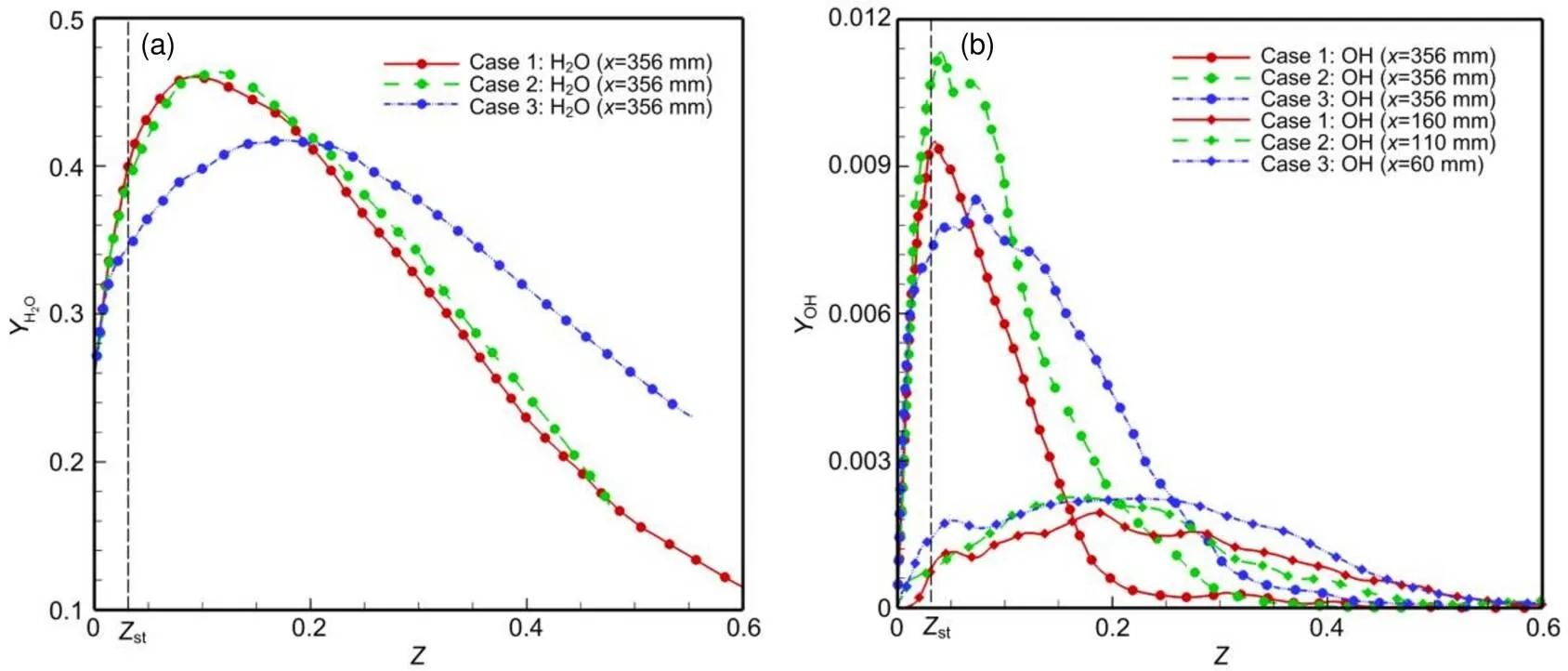
Fig. 17 Quasi-1DH2O (a) and OH (b) mass fraction distributions perpendicular to OH

5 Conclusions

We performed LESs to simulate the wall-jet combustor configuration tested by Burrows and Kurkov, and a stable lifted flame was obtained. The structure of the flow field and the compositions and total temperature profiles at the exit position were in agreement with the experimental results. By analyzing the spatial distribution of compositions and flow parameters, the flame stabilization mechanism was discovered. We carried out further comparisons of different jet total temperatures and observed jet lifted flames with different combustion characteristics. To summarize, the following conclusions can be drawn from this study:

1. The flame is partially premixed and the diffusion flame is dominant. The autoignition cascade controls the stability of the downstream flame: the rich autoignition diffuses to the stoichiometric ratio with increasing flame temperature, forming a stable diffusion flame.

2. The chemical reaction releases heat at the flame lift-off distance and induces local shock waves. The temperature increases after the wave reduces the ignition delay and intensifies the heat release, providing the temperature and heat release conditions to stabilize the lifted flame.

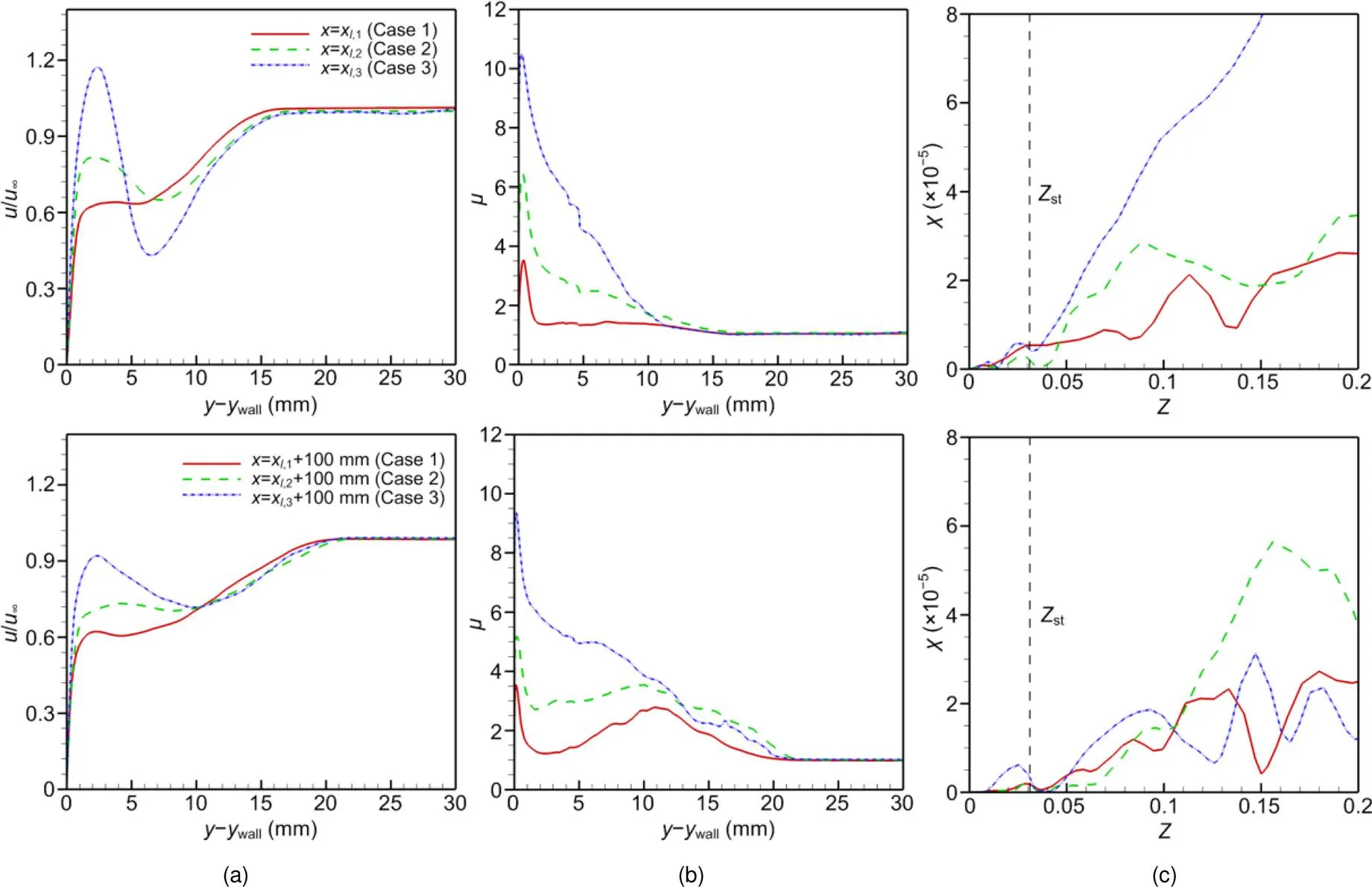
Fig. 18 Velocity (a) and viscosity coefficient (b) distributions in the mixed layer, and scalar dissipation rate distribution (c) with mixture fraction

3. Similar structures are observed under different conditions: mixing zones, autoignition zones, and flame zones. The higher the total temperature, the smaller the flame lift-off distance.

4. In the case with the highest total temperature, the scalar dissipation rate at the stoichiometric ratio exceeds a value that is suitable for the stoichiometric ratio flame, which prevents the completion of the cascade process. Therefore, the flame is mainly fuel- rich rather than concentrated near the stoichiometric ratio, resulting in a low flame temperature.

Contributors

Chao-yang LIU provided the conceptualization and developed the numerical simulation codes. Jin-cheng ZHANG executed the research process and formal analysis, and wrote and revised the manuscript. Hong-bo WANG revised the manuscript and assisted analysis. Ming-bo SUN provided the funding acquisition and resources. Zhen-guo WANG took responsibility for the research.

Conflict of interest

Jin-cheng ZHANG, Ming-bo SUN, Zhen-guo WANG, Hong-bo WANG, and Chao-yang LIU declare that they have no conflict of interest.

Baurle RA, Hsu AT, Hassan HA, 1995. Assumed and evolution probability density functions in supersonic turbulent combustion calculations., 11(6):1132-1138. https://doi.org/10.2514/3.23951

Boivin P, Dauptain A, Jiménez C, et al., 2012. Simulation of a supersonic hydrogen–air autoignition-stabilized flame using reduced chemistry., 159(4): 1779-1790. https://doi.org/10.1016/j.combustflame.2011.12.012

Bouheraoua L, Domingo P, Ribert G, 2017. Large-eddy simulation of a supersonic lifted jet flame: analysis of the turbulent flame base., 179:199- 218. https://doi.org/10.1016/j.combustflame.2017.01.020

Burrows MC, Kurkov AP, 1973. An analytical and experimental study of supersonic combustion of hydrogen in vitiated air stream., 11(9):1217-1218. https://doi.org/10.2514/3.50564

Cheng T, Wehrmeyer J, Pitz R, et al., 1991. Finite-rate chemistry effects in a Mach 2 reacting flow. 27th Joint Propulsion Conference.

Chung SH, 2007. Stabilization, propagation and instability of tribrachial triple flames., 31(1):877-892. https://doi.org/10.1016/j.proci.2006.08.117

Clark RJ, Bade Shrestha SO, 2013. Review of numerical modeling and simulation results pertaining to high-speed combustion in scramjets. Proceedings of the 49th AIAA/ASME/SAE/ASEE Joint Propulsion Conference, p.3724. https://doi.org/10.2514/6.2013-3724

Edwards JR, Boles JA, Baurle RA, 2012. Large-eddy/ Reynolds-averaged Navier–Stokes simulation of a supersonic reacting wall jet., 159(3): 1127-1138. https://doi.org/10.1016/j.combustflame.2011.10.009

Engblom W, Frate F, Nelson C, 2005. Progress in validation of Wind-US for ramjet/scramjet combustion. 43rd AIAA Aerospace Sciences Meeting and Exhibit.https://doi.org/10.2514/6.2005-1000

Förster H, Sattelmayer T, 2008. Validity of an assumed PDF combustion model For SCRAMJET applications. 15th AIAA International Space Planes and Hypersonic Systems and Technologies Conference.https://doi.org/10.2514/6.2008-2585

Frankel SH, Hassan HA, Drummond JP, 1990. A hybrid Reynolds averaged/PDF closure model for supersonic turbulent combustion. 21st Fluid Dynamics, Plasma Dynamics and Lasers Conference.https://doi.org/10.2514/6.1990-1573

Garnier E, Adams N, Sagaut P, 2009. Large Eddy Simulation for Compressible Flows. Springer, Dordrecht, the Netherlands. https://doi.org/10.1007/978-90-481-2819-8

Jachimowski CJ, 1988. An Analytical Study of the Hydrogen-air Reaction Mechanism with Application to Scramjet Combustion. National Technical Information Service, Springfield, Virginia, USA.

Jameson A., 1991. Time dependent calculations using multigrid, with applications to unsteady flows past airfoils and wings. 10th Computational Fluid Dynamics Conference.

Karami S, Hawkes ER, Talei M, et al., 2015. Mechanisms of flame stabilisation at low lifted height in a turbulent lifted slot-jet flame., 777:633-689.https://doi.org/10.1017/jfm.2015.334

Lawn CJ, 2009. Lifted flames on fuel jets in co-flowing air., 35(1):1-30. https://doi.org/10.1016/j.pecs.2008.06.003

Liu CY, Wang ZG, Wang HB, et al., 2016. Mixing characteristics of a transverse jet injection into supersonic crossflows through an expansion wall., 129: 161-173. https://doi.org/10.1016/j.actaastro.2016.09.003

Liu CY, Wang ZG, Wang HB, et al., 2017. Large eddy simulation of cavity-stabilized hydrogen combustion in a diverging supersonic combustor., 42(48):28918-28931. https://doi.org/10.1016/j.ijhydene.2017.09.179

Liu CY, Wang ZG, Sun MB, et al., 2019. Characteristics of a cavity-stabilized hydrogen jet flame in a model scramjet combustor., 57(4):1624-1635. https://doi.org/10.2514/1.J057346

Mastorakos E, 2009. Ignition of turbulent non-premixed flames., 35(1):57-97. https://doi.org/10.1016/j.pecs.2008.07.002

Miake-Lye RC, Hammer JA, 1989. Lifted turbulent jet flames: a stability criterion based on the jet large-scale structure., 22(1):817- 824. https://doi.org/10.1016/S0082-0784(89)80091-8

Moule Y, Sabelnikov V, Mura A, 2014. Highly resolved numerical simulation of combustion in supersonic hydrogen –air coflowing jets., 161(10): 2647-2668. https://doi.org/10.1016/j.combustflame.2014.04.011

O’brien EE, 1980. The probability density function (pdf) approach to reacting turbulent flows.: Libby PA, Williams FA (Eds.), Turbulent Reacting Flows. Springer, Berlin, Germany, p.185-218. https://doi.org/10.1007/3540101926_11

Pitsch H, Desjardins O, Balarac G, et al., 2008. Large-eddy simulation of turbulent reacting flows., 44(6):466-478. https://doi.org/10.1016/j.paerosci.2008.06.005

Star J, Edwards J, Smart M, et al., 2006. Investigation of scramjet flow path stability in a shock tunnel. 36th AIAA Fluid Dynamics Conference and Exhibit.

Sun MB, Wang ZG, Liang JH, et al., 2008. Flame characteristics in supersonic combustor with hydrogen injection upstream of cavity flameholder., 24(4):688-696. https://doi.org/10.2514/1.34970

Vyasaprasath K, Oh S, Kim KS, et al., 2015. Numerical studies of supersonic planar mixing and turbulent combustion using a detached eddy simulation (DES) model.

, 16(4):560-570. https://doi.org/10.5139/IJASS.2015.16.4.560

Wang HB, Sun MB, Wu HY, et al., 2010. Investigation of dual time-step approach for supersonic combustion flow., 32(3):1-6 (in Chinese). https://doi.org/10.3969/j.issn.1001-2486.2010.03.001

Wang HB, Qin N, Sun MB, et al., 2011. A hybrid LES (large eddy simulation)/assumed sub-grid PDF (probability density function) model for supersonic turbulent combustion., 54(10): 2694. https://doi.org/10.1007/s11431-011-4518-6

Wang HB, Wang ZG, Sun MB, et al., 2013. Combustion characteristics in a supersonic combustor with hydrogen injection upstream of cavity flameholder., 34(2):2073-2082. https://doi.org/10.1016/j.proci.2012.06.049

Wang HB, Wang ZG, Sun MB, et al., 2014. Numerical study on supersonic mixing and combustion with hydrogen injection upstream of a cavity flameholder., 50(2):211-223. https://doi.org/10.1007/s00231-013-1227-7

Watson KA, Lyons KM, Donbar JM, et al., 2003. On scalar dissipation and partially premixed flame propagation., 175(4):649-664. https://doi.org/10.1080/00102200302393

Yoon S, Jameson A, 1988. Lower-upper symmetric-Gauss-Seidel method for the Euler and Navier-Stokes equations., 26(9):1025-1026. https://doi.org/10.2514/3.10007

Yoshizawa A, Horiuti K, 1985. A statistically-derived subgrid-scale kinetic energy model for the large-eddy simulation of turbulent flows., 54(8):2834-2839. https://doi.org/10.1143/JPSJ.54.2834

https://doi.org/10.1631/jzus.A2000087

V231

*Project supported by the National Natural Science Foundation of China (Nos. 91741205 and 11522222)

Mar. 5, 2020;

Aug. 31, 2020;

Apr. 6, 2021