Quantification of the impact of environmental factors on chlorophyll in the open ocean*

Dandan ZHAO , Le GAO , Yongsheng XU ,**

1 Key Laboratory of Ocean Circulation and Waves, Institute of Oceanology, Chinese Academy of Sciences, Qingdao 266071, China 2 Laboratory for Ocean and Climate Dynamics, Qingdao National Laboratory for Marine Science and Technology, Qingdao 266071, China

3 University of Chinese Academy of Sciences, Beijing 100049, China

4 Center for Ocean Mega-Science, Chinese Academy of Sciences Qingdao 266071, China

Abstract Many previous studies of the impact of oceanic environmental factors on chlorophyll (CHL)in a specific region focused on sea surface temperature (SST), mixed-layer depth (MLD), or wind stress(WS) alone. In this study, relationship between CHL and all those environmental factors (SST, MLD, and WS) in the open ocean was quantified for five regions within the subtropical gyres and the variation trend of 13-year (2003-2015) was analyzed using satellite observations and Argo measurements. The correlation analysis results show that MLD was correlated positively with CHL, SST was correlated negatively with CHL, and the correlation between CHL and WS was either positive or negative. Based on the significance of the correlations, models representing the relationships were established using the multiple linear regression and analyzed, showing that the environmental factors were the major determinants of CHL change. The regression coeffi cients show that both SST and MLD have remarkable eff ect on CHL. Our derived models could be used to diagnose the past changes, understand present variability, and predict the future state of CHL changes based on environmental factors, and help us understand the dynamics of CHL variation in the open ocean.

Keyword: chlorophyll (CHL); mixed layer depth (MLD); multiple linear regression; sea surface temperature (SST)

1 INTRODUCTION

Chlorophyll (CHL) is the principal globally available indicator of ocean primary production, and CHL variation is closely related to the changes in the oceanic physical environment. One of the most important issues in studying the dynamics of ocean CHL is the analysis of environmental factors that control the growth of CHL (Raymont, 1980).Therefore, CHL could potentially provide a globalscale assessment of possible links between productivity and physical changes (Killworth et al.,2004; Behrenfeld et al., 2006). The oceanic CHL concentration, which represents phytoplankton biomass, can be observed by ocean color remote sensing. However, such remote sensing measurement can be conducted during daylight hours only, and it is much more challenging for those of the environmental factors. The primary limitation is the data gaps owing to the inability to measure ocean color when clouds are present. The secondary limitation is the noisiness of the CHL fields due to water-leaving radiance,which is estimated for ＜10% of the total visible radiance measured by satellites. Furthermore, satellite measurements must be corrected for atmospheric contamination and other eff ects prior to estimation of the CHL concentration (Chelton et al., 2011a). Earlier analyses of surface CHL in the subtropical gyres have been performed for short periods of the SeaWiFS record (McClain et al., 2004). Analysis of recent trends in global ocean CHL (1998-2003) has shown an overall of 4.1% global trend ofincrease in surface CHL (Gregg et al., 2005). The dynamics of remotely sensed phytoplankton biomass in Santa Monica Bay and the adjacent San Pedro Basin, analyzed using the wavelet method, have revealed evident seasonal patterns of variation (Nezlin and Li, 2003). Previous studies have found that sea surface temperature (SST)has an important impact on the distribution of CHL(Kavak and Karadogan, 2012; Ji et al., 2018).Furthermore, fluctuations in the mixed-layer depth(MLD) in relation to CHL variability have been investigated in the Kuroshio-Oyashio extension region (Itoh et al., 2015), and the eff ect of wind stress(WS) on the distribution of oceanic CHL has also been investigated (George and Edwards, 1976; D’Sa and Korobkin, 2009).

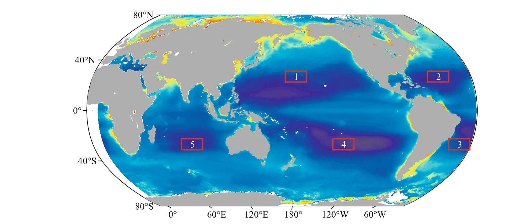
Fig.1 Regions defined by coherent distribution of 4-km grid points where chlorophyll (CHL) concentration was ≤0.1 mg/m 3 during 2003–2015 and bottom depth was ≥1 000 m

The variability of CHL in the surface waters of the open ocean is associated with SST, WS, and MLD, as well as many other oceanic environmental factors.The primary environmental factors (i.e., SST, MLD,and WS) may be envisioned as input to a black box whose output is the observed CHL variability. As there might be more than one possible outcome in a multivariate system, it is imperative to understand clearly the relationships between the dependent variable (chl) and the independent variables (sst, mld,and ws). In this study, we focused on five regions within the subtropical gyres (red boxes in Fig.1;bottom depth＞1 000 m). The chosen regions are oligotrophic areas (McClain et al., 2004), and the upper of them is primarily wind driven (Huang and Russell, 1994). Ignoring the influence oflight, we concentrated on the influence of physical environmental factors. In the five selected regions,the surface CHL concentration during a 13-year period (2003-2015) was ≤0.1 mg/m3.

Based on satellite retrievals and Argo observations,we investigated the relationships between oceanic CHL and certain environmental factors in the selected regions. The objectives of the work were as follows:(1) to determine the trends of CHL, SST, MLD, and WS in the selected regions; (2) to calculate the correlations between CHL and SST, WS, MLD on the monthly timescale during 2003-2015; and (3) to construct models using multiple linear regression to quantify the relationship between CHL and a set ofindependent variables (i.e., SST, MLD, and WS).

2 DATA AND METHOD

Satellites provide continuous and long-term observations of global ocean CHL and wind speed from space. Argo is a global array of 3 800 freedrifting oceanic profiling floats that provide vertical profiles of temperature and salinity in the upper 2 000 m. These data are subject to real-time quality control. Satellite-derived wind speed data are retrieved using two scatterometers: the SeaWinds Kuband scatterometer onboard the QuikSCAT satellite and the C-band ASCAT. In the two and half years of ASCAT/QuikSCAT overlap, the wind speed datasets were processed in a consistent manner using a radiative transfer model and careful instrument intercalibration (Wentz, 1997; Bentamy et al., 2012).Concurrent CHL, SST, and WS datasets are treated in the same manner to obtain 1°×1° monthly values. WS is connected to the production of wind-driven surface currents and upper-ocean mixing (Pond and Pickard,1978; Uz and Yoder, 2004), and wind speed is converted into WS as a function of wind speed, a nondimensional drag coeffi cient, and boundary-layer air density. Although MODIS-Aqua began collecting data in July 2002, we only used data from 2003-2016 because complete annual records from MODIS-Aqua were available for this period together with concurrent SST, wind speed, and Argo datasets.

First, the trends were assessed using the following methods.

(1) The monthly anomaly ( y) is generated by subtracting the monthly mean values from each month to eliminate the influence of the background field(Gregg et al., 2005). With y representing the mean value of the monthly anomalies during 2003-2015,the standardized data ( y*) were calculated as Eq.1:

where σyis the standard deviation of the monthly anomalies. The purpose of this data standardization technique was to eliminate the influence of the noise of the variables.

(2) The best-fit linear trend was then computed using linear regression analysis.(3) The statistically significant trend was displayed as the one that exceeded the 95% confidence level, the correlation between CHL and the three environmental factors was calculated, and the relationships between CHL and the environmental factors were determined using multiple linear regression analysis.

3 RESULT

3.1 Monthly variation of CHL and environmental factors

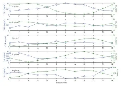
Fig.2 Variations of monthly averages (2003–2015) of SST, MLD, WS, and CHL in Regions 1-5

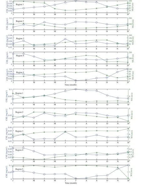
Fig.2 Continued

Table 1 Slope and intercept of the trend line of CHL, SST, MLD, and WS in Regions 1–5 and the global ocean (slope; intercept)

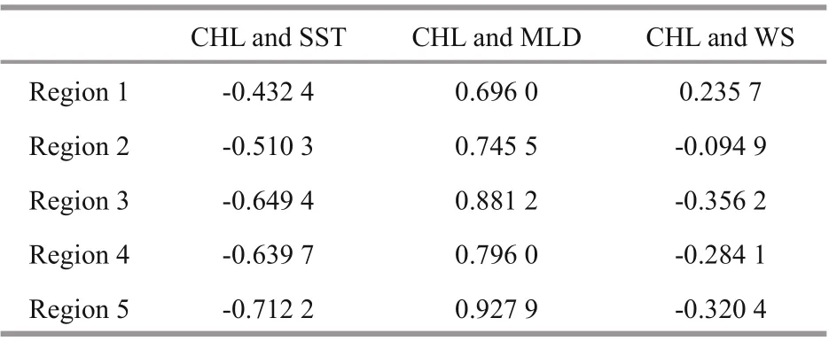
Table 2 Correlation coeffi cients between CHL and SST,MLD, and WS in Regions 1–5

Temporal analysis of the monthly averages CHL and the environment factors during 2003-2015 for our selected regions was performed. Although Regions 1 and Region 2 (or Regions 3-5) are located at the same latitudinal band, the variation of SST is diff erent. As seen in Fig.2, the SST of Region 1 shows an upward trend during January-March, a downward trend during March-September, and a further upward trend until December. In Region 2, SST increases during January-February, decreases during February-August, and increases during August-December. The SST of Region 3 decreases during January-February,increases during February-May, decreases slightly in June, increases during June-October, and then decreases until December. The pattern of SST variation in Region 4 is the opposite of that in Region 1. The patterns of change of SST in Region 5 is increase-decrease-increase-decrease. We found that the depth of the mixed layer was largely in the range of 20-100 m. The depth of the mixed layer in Regions 1 and 2 increases during January-February and decreases during February-June and increases until December. However, in Regions 3 and 4, it increases during January-August and then decreases during November-December. The changes of CHL and wind speed in each region are also diff erent. The above analysis show that the seasonal patterns of CHL and environmental factors changes are not obvious.

3.2 Trends in the selected regions

A 13-year time series of CHL was evaluated using linear regression analysis to assess the recent trend based on satellite observations from 2003-2015(Fig.3). In the five selected regions, noteworthy positive trends of CHL are apparent in Regions 3-5,whereas the trends in Regions 1 and 2 are negative,and the seasonal cycle of CHL is obvious (Fig.3,Table 1). Regions 1 and 2 have increasing trends in SST and WS but decreasing trends in MLD. Increasing trends in MLD are observed in Regions 3-5 but the SST exhibits a trend of decrease. Regions 4 and 5 show a trend of decrease in WS, while Region 3 has a trend ofincrease. Higher ocean temperatures can produce a shallower mixed layer, allowing greater light availability in the mixed layer. A shallower upper MLD will probably lead to increased nutrient limitation and reduced nutrient exchange with deeper layers. We also calculated the slope and intercept of the trend line of the global CHL. Global CHL has an upward trend (Table 1), which is consistent with the results of Gregg et al. (2005) who reported an overall of 4.1% global increase in CHL for the same period.

3.3 Correlations between CHL and the environmental factors

The correlations between CHL and the environmental factors were analyzed based on monthly observation datasets. Determining those environmental factors that are correlated with CHL is beneficial for understanding their interactions. The movement of the upper-level water of the selected regions primarily reflects a wind-driven circulation.The salinity and temperature provide the opportunity to calculate the density gradient. As the horizontal density gradient increases, the pycnocline and the nutriclines deepen, which influences the CHL concentration. Thus, the distribution of CHL is related to oceanic environmental factors (e.g., SST, MLD,and WS). The correlation between CHL and SST is negative in each selected region (Table 2). This might be because temperature influences CHL growth directly through its eff ect on the metabolic rate of organisms (Gregg et al., 2005; Feng et al., 2015).However, higher temperatures shorten the turnover times of plankton, produce a shallower MLD, and limit the nutrient supply. Thus, SST can regulate oceanic CHL indirectly (Gregg et al., 2005). The MLD is correlated positively with CHL, whichindicates nutrient limitation (Lovenduski et al., 2008;Fay and Mckinley, 2017). Our results reveal that WS is an important factor in explaining the variance of CHL. The correlation coeffi cient between CHL and WS in Region 1 is positive, whereas it is negative in the other selected regions. The interesting correlation between CHL and WS is because some of the correlation is due to the direct influence of wind forcing on CHL, while some is due to the indirect influence of wind forcing on CHL. Upwelling or downwelling driven by the variability of winds aff ects the supply of nutrients, and therefore leads to an increase or decrease in CHL (Webster and Hutchinson,1994; Wang et al., 2013), which illustrates the indirect eff ect of wind on CHL.

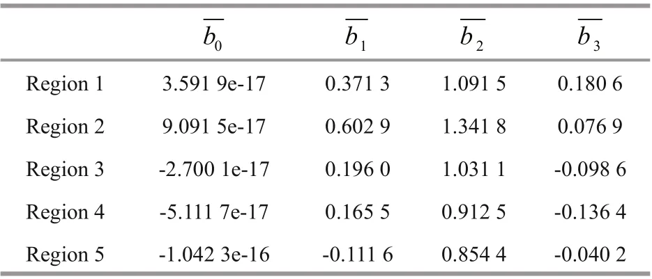
Table 3 Standardization regression coeffi cients for Regions 1–5

3.4 Analysis of the impact of the environmental factors on CHL

Analysis of the environmental factors controlling CHL variability is an important scientific issue.Various methods including laboratory experiments and mathematical simulations are used to investigate the mechanisms via which such factors might influence CHL (Nezlin and Li, 2003). However,although it is known that CHL might be influenced by various independent variables (e.g., SST, MLD, and WS), exactly how these environmental factors might aff ect CHL is not yet fully understood. The correlation analysis described above found CHL correlated significantly with SST, MLD, and WS. In the following, the direct relationship between CHL and these environmental factors is explored using the multiple linear regression method based on observation datasets.

The dependent variable (chl) can be denoted approximately as the linear function ofindependent variables (sst, mld, and ws). The full model incorporates by monthly environmental factors (sst,mld, and ws) eff ects as Eq.2:

where b0is a constant, b1, b2, b3are partial regressioncoeffi cients, (chl)t, (sst)t, (mld)t, and (ws)tare the monthly time series ( t=1, 2, 3, ···, 156) of chl, sst,mld, and ws, the residual (err)tis the random error that excludes three entries independent variable influence to (chl)t. We first need to standardize each independent variable (sst, mld, and ws) and dependent variable(chl) for comparison with the eff ective intension of each independent variable (sst, mld, and ws) to chl.Modeling the impact of the environmental factors on CHL will allow us to simultaneously capture the linear eff ects of several variables. This model is used to explore the direct relationships between oceanic CHL and the environmental factors. Using the standardized data, the regression can be derived as follows:

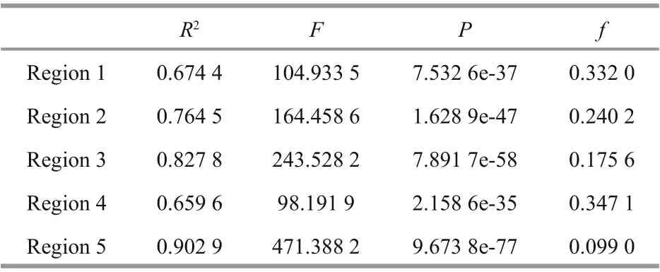
Table 4 Estimates of the error variance in Regions 1–5

and the corresponding regression coeffi cient is the standardization regression coeffi cient. If the absolute value of the standardization regression coeffi cient is large, the corresponding independent variable has large influence on the dependent variable (chl). The regression coeffi cients b0, b1, b2, and b3, are shown in Table 3. The absolute values of b1are greater than b3,and b2responds to b3in a similar manner, which means CHL is aff ected more by SST and MLD than by WS. The results of the multiple linear regression analysis are presented in Fig.4. After fitting the regression line, it is important to investigate the residuals to determine whether they appear to fit the assumption of a normal distribution. The normal cumulative distribution of the residuals is shown at the right of each panel in Fig.4. An estimate of the error variance is shown in Table 4. The result for each region in the Southern Hemisphere is better than for the regions in the Northern Hemisphere. This might be because CHL in the Northern Hemisphere might be influenced more by factors that have been ignored,e.g., coastal upwelling, eddy-induced CHL transport,local precipitation, and the change of weather.However, the results indicate that SST, MLD, and WS are important factors in controlling the distribution of oceanic CHL, especially SST and MLD.

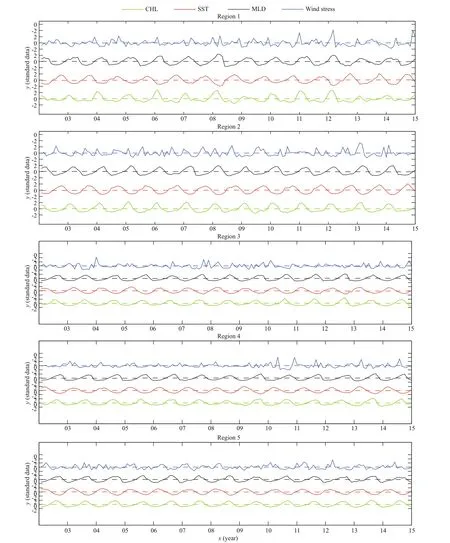
Fig.3 Time series of CHL, SST, MLD, and WS anomalies in Regions 1–5

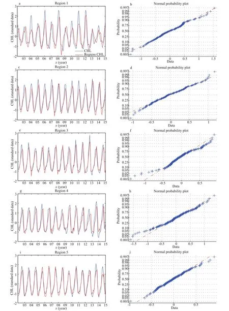
Fig.4 Relational model between CHL and SST, MLD, and WS for Regions 1–5

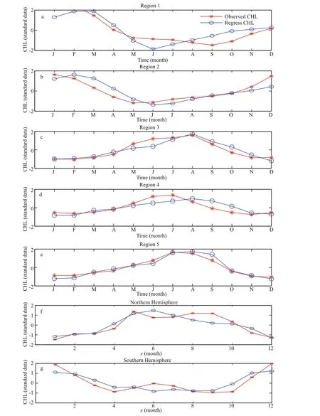
Fig.5 Model validation based on satellite-derived data of 2016

Satellite-derived data of 2016 were used to validate our models and to determine whether the models respond well to the relationship between CHL and the environmental factors. The anomalies of CHL, SST,MLD, and WS were computed using Eq.1. The satellite-observed CHL and that calculated using our models in the selected regions are shown in Fig.5. It can be seen that our models display satisfactory capability in depicting the relationship between CHL and the environmental factors in our selected regions.We tested the applicability of our models to the Northern Hemisphere, and the regression coeffi cients we chose were the averages of the regression coeffi cients for Regions 1 and 2. A similar methodology was adopted for the Southern Hemisphere. Overall,although the simulation results for the Northern(Southern) Hemisphere are less satisfactory than for the individual regions, they still capture the main change of CHL over time (Fig.5f & g).

4 DISCUSSION AND CONCLUSION

Many previous studies that focused on elucidating the impact of environmental factors on CHL considered only a single variable (i.e., SST, WS, or MLD) or only specific regions (George and Edwards,1976; D’Sa and Korobkin, 2009; Kavak and Karadogan, 2012; Itoh et al., 2015; Ji et al., 2018).The referenced studies found that some physical processes (e.g., upwelling and mixing) drive the changes in oceanic CHL. The influence of physical processes on CHL is complex and the eff ects of environmental factors on CHL are interdependent.For example, as the regions we selected for this study are subject to wind forcing, their circulation strength will be adjusted accordingly. As the circulation strengthens, the horizontal density gradient will increase and both the pycnocline and the nutriclines will deepen. All these changes include variations in SST, MLD, and WS that work together to drive changes of CHL. Coupling between environmental factors complicates the problem. In our study, it is assumed that the eff ects of these environmental factors on CHL are independent. We selected five representative regions within the subtropical gyres,and developed models to describe the relationship between surface CHL and certain environmental factors. We analyzed the time series of anomalies in remote-sensed surface CHL concentration and their associated environmental factors. Regions 1 and 2 exhibited reasonably weak downward trends in CHL,whereas Regions 3-5 showed weak upward trends.Correlation analysis revealed significant relationships between CHL and the environmental factors. It was found that MLD (SST) was correlated positively(negatively) with CHL. Our regression coeffi cients showed that SST and MLD both had remarkable eff ect on CHL. Our model could be used to diagnose past change, understand present variability, and predict the future state of CHL changes based on environmental factors in the open ocean, which could help us develop greater understanding of the eff ect of these environmental factors on the distribution of oceanic CHL.

Although SST, MLD, and WS are the principal environmental factors controlling changes of CHL, in a realistic oceanic environment (Gregg et al., 2005;McQuatters-Gollop et al., 2008; Liu et al., 2012; Ji et al., 2018), ocean carbon absorption (Lovenduski et al., 2008; Fay and McKinley, 2017) could play an important role in changes of CHL. If ocean carbon absorption were considered, it could improve the accuracy of our models.

5 DATA AVALABILITY STATEMENT

The global CHL data is downloaded from (https://oceandata.sci.gsfc.nasa.gov/MODIS-Aqua/Mapped/Monthly/4km/chlor_a). SST data used in this study is available at (https://oceandata.sci.gsfc.nasa.gov/MODIS-Aqua/Mapped/Monthly/4km/sst). MLD is obtained from Argo data, the Argo data can be downloaded from (http://www.usgodae.org/argo/argo.html). Wind data can be downloaded from(http://www.remss.com/).