Typhoon wind hazard model and estimation on return period of typhoon wind speed*

Yunxia GUO, Yijun HOU , Peng QI

1 Key Laboratory of Ocean Circulation and Waves, Institute of Oceanology, Chinese Academy of Sciences, Qingdao 266071,China

2 University of Chinese Academy of Sciences, Beijing 100049, China

3 Laboratory for Ocean and Climate Dynamics, Qingdao National Laboratory for Marine Science and Technology, Qingdao 266237, China

4 Center for Ocean Mega-Science, Chinese Academy of Sciences, Qingdao 266071, China

Abstract Typhoons are one of the most serious natural disasters that occur annually on China’s southeast coast. A technique for analyzing the typhoon wind hazard was developed based on the empirical track model, and used to generate 1 000-year virtual typhoons for Northwest Pacific basin. The influences of typhoon decay model, track model, and the extreme value distribution on the predicted extreme wind speed were investigated. We found that diff erent typhoon decay models have least influence on the predicted extreme wind speed. Over most of the southeast coast of China, the predicted wind speed by the nonsimplified empirical track model is larger than that from the simplified tracking model. The extreme wind speed predicted by diff erent extreme value distribution is quite diff erent. Four super typhoons Meranti(2016), Hato (2017), Mangkhut (2018), and Lekima (2019) were selected and the return periods of typhoon wind speeds along the China southeast coast were estimated in order to assess the typhoon wind hazard.

Keyword: typhoon; empirical track model; decay model; extreme wind speed; return period

1 INTRODUCTION

China’s southeast coast is the region of the world that suff ers most from severe typhoon disasters.Typhoons, known as hurricanes in the eastern Pacific and Atlantic oceans, can create complex environments of high winds, heavy rainfall, huge wave heights, and huge storm surges throughout the region. Therefore, it is very important to analyze the typhoon hazard risk using typhoon wind hazard modeling and simulation methods.

In the second half of the 20thcentury, the Monte Carlo simulation was adopted most widely for performing typhoon risk analysis. It uses a typhoon wind field model and typhoon history data to simulate the typhoon wind field and to predict the annual maximum wind speed. Both the United States(American Society of Civil Engineers, 2005) and Australia (Standards Association of Australia, 2002)use the method to compile design wind speed maps.

The simulation approach was first implemented by Russell (1968, 1971) for the Texas coast (USA). Since that pioneering study, the modeling technique has been expanded and improved by Batts et al. (1980),Shapiro (1983), Georgiou et al. (1983), Vickery and Twisdale (1995b), Meng et al. (1995), Simiu and Scanlan (1996), and Thompson and Cardone (1996).As indicated by Vickery and Twisdale (1995a),although the approaches used by these investigators are similar, there are significant differences in the decay models, wind field models, size of the region over which the typhoon climatology can be considered uniform, and use of a coast segment crossing approach.

Since 2000, the full-track modeling method has gradually been developed (Vickery et al., 2000, 2009;Huang et al., 2001; James and Mason, 2005; Hall and Jewson, 2007). Vickery et al. (2000) are pioneers of full-track modeling and they developed an empirical track model. This model can generate the full track of a tropical cyclone (TC) from generation to extinction.As indicated by Vickery et al. (2000), an improvement of the storm track modeling approach over a Monte Carlo simulation is that it is not dependent on the hypothesis of climate uniformity in the subregion.Therefore, even in a large region with considerable change in typhoon climatology, it remains appropriate for typhoon hazard analysis, which is helpful for analyzing the risk oflarge-scale systems. The empirical track model has been used in many studies for typhoon hazard analysis (Powell et al., 2005; Lee and Rosowsky, 2007; Legg et al., 2010; Apivatanagul et al., 2011; Li and Hong, 2014, 2016; Pei et al.,2014). The design wind speeds recommended by U.S.building codes (American Society of Civil Engineers,2010) are also based on the empirical track model(Vickery et al., 2000). Recently, a track model based on statistical dynamics method has been proposed(Emanuel, 2006; Emanuel et al., 2006; Chen and Duan, 2018) which performs well in both TC-rich and TC-rare areas.

The process of analyzing typhoon risk using the empirical track model is that first a large number of virtual typhoons is generated using the typhoon empirical track model. Then, the typhoons that aff ect a certain research site are extracted from the virtual typhoons using the simulated circle method. Next, a typhoon wind field model is used to calculate the wind speed of the extracted typhoons, from which samples of maximum wind speed can be derived.Finally, the samples of maximum wind speed are fitted by some extreme value distribution, based on which extreme wind speeds for diff erent return periods can be predicted. Many factors can influence the prediction of extreme wind speed throughout the entire process. The empirical track model developed by Vickery et al. (2000) was simplified by Li and Hong (2014) through the adoption of the geographic weighted regression method (Fotheringham et al.,2002), and they also fully validated the effi ciency of the simplified tracking model. Vickery (2005) also developed a new model for hurricane decay after landfall.

In this paper, we investigated the sensitivity of the typhoon wind hazard model to diff erent influencing factors including diff erent typhoon decay models, the simplified and non-simplified typhoon tracking models, and diff erent extreme value distributions.The eff ects of these factors on predicted extreme wind speed for 50-year and 100-year return periods in the southeast coastal region of China are explored quantitatively. Besides, we select four super typhoons Meranti (2016), Hato (2017), Mangkhut (2018),Lekima (2019), and estimate the return periods of typhoon wind speeds along the China’s southeast coast to assess their risk.

2 EMPIRICAL TRACK MODEL

Vickery et al. (2000) developed the typhoon empirical track model, which models the typhoon translation speed, storm heading, and relative intensity. The model is expressed as:

where coeffi cients ai, bi, and diare developed on a 5°×5° grid over the entire Northwest Pacific basin,based on regression analysis of historical typhoon data; Ψ and λ represent the storm latitude (°) and longitude (°), respectively; ci, θi, and Iiare the typhoon translation speed, storm heading, and relative intensity, respectively, at time step ofi; Δln c=ln ci+1−ln ci; Δ θ= θi+1− θi; T siis monthly mean sea surface temperature ( K); and εc, εθ, and εIare random error terms. The historical typhoon dataset used here is the China Meteorological Administration-Shanghai Typhoon Institute Best Track Dataset for Tropical Cyclones over the Western North Pacific (1949-2017,from www.typhoon.gov.cn).

The relative intensity I is defined as (Darling, 1991):

where pdaand pdcare the ambient and minimum sustainable central dry partial pressures, respectively,and Δ p is the central pressure difference. For details on the specific method for the calculation of relative intensity, the reader is referred to Darling (1991). We distinguish easterly and westerly headed storms, and we obtain two set of coeffi cients ( ai, bi, and di) for both types. When a grid cell has few or no historical typhoons, the coeffi cients are replaced with those of the nearest grid cell.

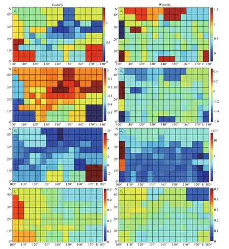
Fig.1 Illustration of regression coeffi cients a in Eq.3 for easterly (left) and westerly (right) headed storms

In the tracking model of Vickery et al. (2000),many coeffi cients have to be determined for each grid cell. Li and Hong (2014) eliminated some secondary explanatory variables in the regression model and they simplified the tracking model of Vickery et al.(2000) using the geographic weighted regression method (Fotheringham et al., 2002). The simplified tracking model can be expressed as follows:

Li and Hong (2014) compared the standard deviations of the residuals in the regression analysis for Eqs.1 & 3 and they indicated that the fit obtained by Eq.3 is comparable with Eq.1. In this study, the simplified tracking model is used and the fitting coeffi cient aiin Eq.3a is illustrated in Fig.1 from which we can observe its spatial variation. Those for the other coeffi cients in Eq.3 are not shown because of space limitations.

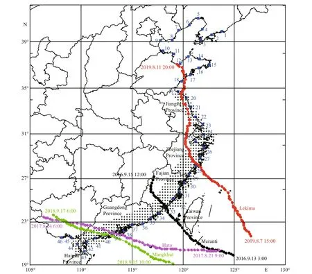
Fig.2 Locations of 46 coastal stations (blue squares) along China’s coastline, 579 research points (black asterisks), and tracks of Typhoons Meranti, Hato, Mangkhut, and Lekima

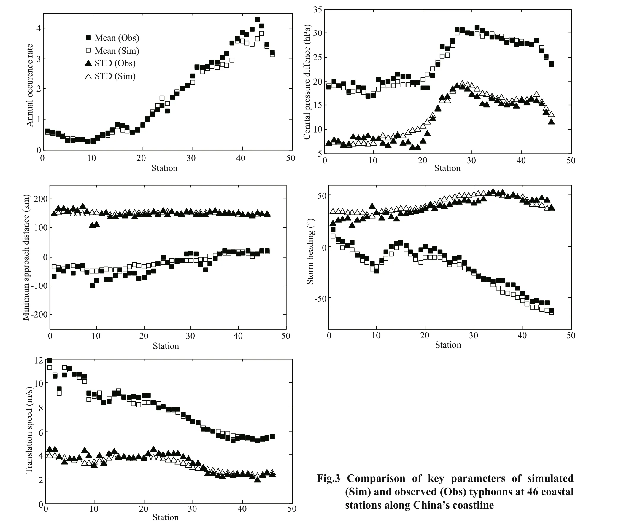
Before using the empirical track model, we need to validate its effi ciency. Firstly, virtual typhoon events over 1 000 years in the Northwest Pacific basin are simulated using Eq.3. The historical typhoon data used for verification are obtained from the China Meteorological Administration dataset. Overall, 46 coastal stations are selected along the coast of China,as shown in Fig.2 (blue squares). In addition, the distance between the adjacent stations equals about 100 km. Then, the typhoon events aff ecting each station (i.e., typhoons that pass within 250 km) are extracted from the virtual and historical typhoons datasets. The use of a 250-km subregion has been suggested by Li and Hong (2015, 2016) and by Vickery et al. (2009) following parametric investigation. Next,statistics such as mean annual occurrence rate, the mean and standard central pressure difference,minimum approach distance, translation speed, and storm heading are obtained for the simulated and historical tracks. All the values of these key parameters(except the central pressure difference) are obtained when they are closest to the coastal station. The central pressure difference is estimated using the minimum values within the 250 km subregion. When a typhoon passes to the right (left) of a site, the minimum approach distance is considered positive (negative).

Figure 3 compares key parameters of typhoons simulated by Eq.3 and observed typhoons along China’s coastline. The figure shows that the characteristics of simulated typhoons are in good agreement with those from the observational dataset,which indicates that empirical track model can reproduce the characteristics of typhoons along China’s coastline.

3 SENSITIVITY OF TYPHOON WIND HAZARD MODEL

The empirical track model is mainly used to generate large numbers of virtual typhoons to analyze the typhoon risk. Many factors can influence the prediction of extreme wind speed throughout the entire process, e.g., diff erent typhoon tracking models,diff erent typhoon decay models, and diff erent extreme value distributions. To explore the sensitivity of the typhoon wind hazard model to the above factors, we calculate the extreme wind speeds (representing 10-min mean wind speed at 10 m height) for diff erent return periods under the influence of diff erent factors and make a comparison. To map the typhoon wind hazard, we select 579 grid points as research sites in the southeast coastal region of China, as shown in Fig.2 (black asterisks). The grid resolution is set to 0.25°, and for each research site, the extreme wind speeds at 50- and 100-year return periods are predicted under the influence of the diff erent factors.

The Yan Meng (YM) wind field model, developed by Meng et al. (1995), is applied in this study to calculate the wind speed. As indicated by Meng et al.(1995), the model involves moving wind field model of typhoons and introduces the concept of the“equivalent roughness length” to consider topographical eff ects. The YM model is suffi ciently accurate for typhoon simulation and it has been applied by Matsui et al. (2002), Zhao et al. (2005),and Xie et al. (2015).

The equation of motion in YM model can be written as:

Table 1 Decay constant a in Eqs.6 & 7

where ρ is the air density, k is the vertical unit vector, fis the Coriolis parameter, V is the typhoon-induced wind velocity. In the YM model, V is decomposed into the gradient wind Vgin the free atmosphere and the friction wind V´. Iterated computation is used to solve the YM wind field model. More details about the wind field model can be found in Meng et al. (1995).

The pressure model used in this study is from Holland (1980):

where p( r) is the surface pressure at a distance r from the typhoon center, p0is the central pressure, Δ p is the central pressure deficit, B is the pressure profile constant, the range is estimated to be 0.5-2.5, Rmaxis the radius to maximum winds. The wind speed calculated by the YM model is an hourly mean and the ratio of the maximum 10 min mean wind speed to the hourly mean is equal to 1.06.

3.1 Influence of diff erent decay models on extreme wind speeds

When a typhoon makes landfall, its intensity will weaken because of the loss of energy from the sea and the increased ground friction. Modeling the decay of typhoons after landfall plays an important role in typhoon risk analysis at coastal stations. We first investigate the influence of the typhoon decay model on predicted wind speed. The simplified empirical track model is used to generate virtual typhoon events in the Northwest Pacific basin, and in this process, we apply two diff erent decay models. One is the model developed by Vickery and Twisdale (1995b):

where Δ p( t) is the central pressure difference (hPa) at time t after landfall, Δ p0is the central pressure difference (hPa) at landfall, a is the decay constant,and ε is a normally distributed error term. The other model is the model developed by Vickery (2005):

where c is the typhoon translation speed at landfall(km/h), and Rmaxis the radius to maximum winds at landfall (km). Vickery (2005) indicated that Eq.7 can increase the correlation coeffi cient R2in regression analysis (coeffi cients a0and a1are determined by regression analysis) on the Gulf Coast, Florida Peninsula, and Atlantic Coast of the USA.

The typhoon landing area in the Northwest Pacific basin is divided into five subregions: the region north of 30°N (extratropical cyclone area, Zone1), region between 25°N and 30°N (area north of Taiwan, China,Zone2), region between 20°N and 25°N (area including Taiwan, China, Zone3), region of The Philippine Islands (Zone5), and region of the remaining areas(Zone4). The fitting coeffi cients of Eqs.6 & 7 are summarized in Table 1, where N is the number of data points used for the regression analysis and σεis the standard deviation of the errors. In Table 1, the largest value of R2is shown in bold for each region examined.It can be seen that the correlation in the decay model of Vickery and Twisdale (1995b) is better than that of Vickery (2005) for most regions.

In Section 2, we use the simplified empirical track model and the decay model of Vickery and Twisdale(1995b) to generate virtual typhoons and validate their statistical characteristics. Here, we use the same track model but with the new decay model of Vickery(2005) to generate virtual typhoons for the Northwest Pacific basin and validate its effi ciency. Because of space limitations, the results of the verification are not given here. The numerical experiment using Eqs.3 &6 to predict the wind speed is referred to as Test 1, and that using Eqs.3 & 7 is referred to as Test 2.

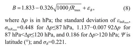
In this paper, the Rmaxand B in the wind field model are calculated based on the models given in Vickery and Wadhera (2008) (see also Eqs.5 & 6 in Li and Hong (2015)):

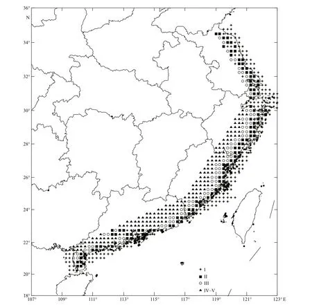
Fig.4 The roughness length for each research site

In Meng et al. (1995), the terrain roughness and topographical eff ect were expressed by a single roughness length. The values of the roughness length for diff erent geomorphology based on past studies(Counihan, 1975; Standards Association of Australia,2002; Choi and Kanda, 2010) are shown in Table 2.

We marked the roughness length for each research site according to the topography and the results are shown in Fig.4.

The empirical distribution is used as the extreme value distribution in both Test 1 and Test 2. Table 3 shows the settings for Tests 1 and 2 as well as other tests described in the following section of this paper.

The predicted extreme wind speeds for a 50-year return period ( V50) for 579 sites in the southeast coastal region of China are used to map the typhoon hazard, as shown in Fig.5 (a, Test 1) and (b, Test 2). It can be seen from Fig.5 that the diff erent decay models,i.e., Eqs.6 & 7, have little impact on the predicted wind speed, and that the maximum difference (MD)of wind speed is only about 1.0 m/s. We also compare the predicted wind speeds for a 100-year return period( V100) for Tests 1 and 2 (not shown because of space limitations). The MD is also about 1.0 m/s and the maximum relative difference (MRD) is only about 3%.

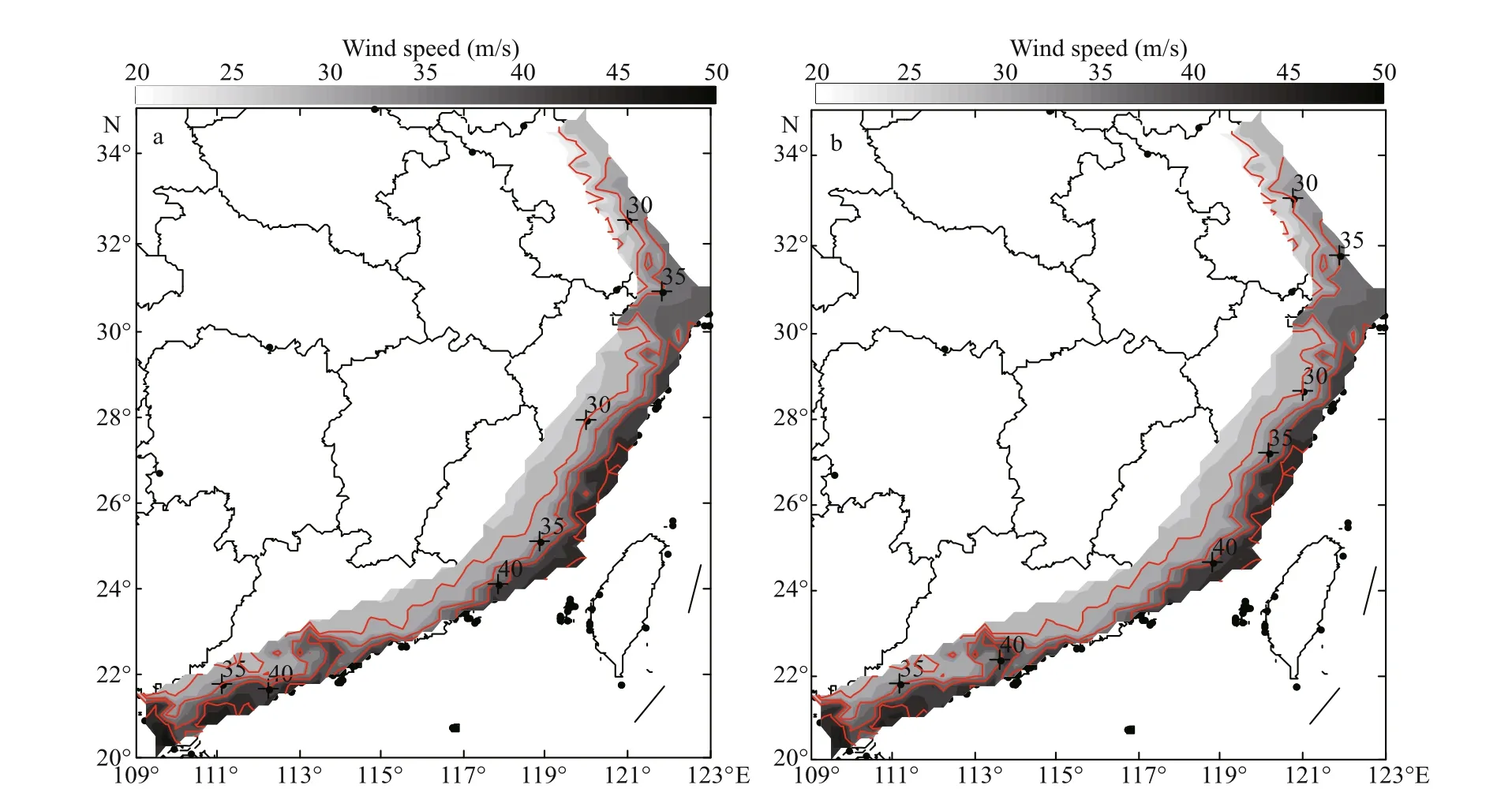
Fig.5 Maps of extreme wind speeds (m/s) for 50-year return period in Test 1 (a) and Test 2 (b)

Table 2 Roughness length (m) of diff erent geomorphology

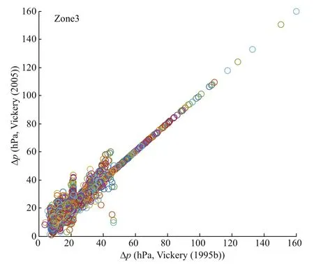
Fig.6 Scatter plot of the typhoon pressure difference at all times obtained by the Vickery and Twisdale (1995b)and Vickery (2005) decay models for the typhoons landing in Zone3

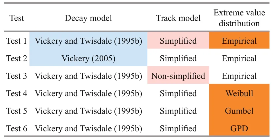
Table 3 Settings for diff erent tests

In order to analyze how diff erent decay models cause the difference of predicted wind speed, we use Eqs.6 and 7 to calculate the central pressure difference for the landing typhoons constructed by the simplified track model and compare them. Figure 6 shows the scatter plot of the typhoon pressure difference at all times obtained by the two decay models for the typhoons landing in Zone3. The X-axis and Y-axis represent the results of Vickery and Twisdale (1995b)and Vickery (2005) decay models respectively. It can be seen from Fig.6 that most of the scatters are distributed around a straight line with a slope of 1,indicating that the central pressures obtained by the two diff erent decay models have little difference. This explains why the two diff erent decay models have little impact on the predicted wind speed in Fig.5. For the other four typhoon landing areas, we also carry out a similar analysis, and the results are similar to those of Zone3.

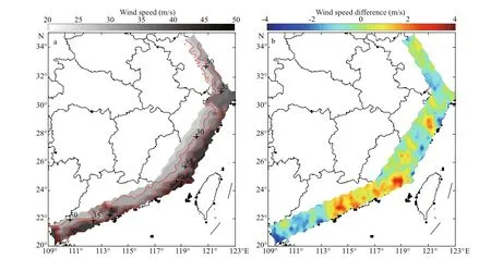
Fig.7 Maps of extreme wind speeds (m/s) for 50-year return period in Test 3 (a) and the wind speed difference (m/s) between Tests 3 and 1 (b)

3.2 Influence of diff erent track models on extreme wind speeds

To investigate the influence of the non-simplified and simplified track models on predicted extreme wind speeds, we estimate V50and V100for China’s southeast coast based on the virtual typhoons generated using Eqs.1 & 2. In this process, the decay model of Vickery and Twisdale (1995b) and the empirical distribution are adopted. The numerical experiments are referred to as Tests 1 and 3, as shown in Table 3. The predicted V50in Test 1 is shown in Fig.5a. The estimated V50in Test 3 is shown in Fig.7a and the wind speed difference between Tests 1 and 3 is shown in Fig.7b. It can be seen from Fig.7b that the wind speeds predicted by the non-simplified track model (Test 3) are larger than those predicted by the simplified track model (Test 1) in the coastal regions of northern Guangdong and Fujian provinces. The MD of predicted wind speed is about 3.5 m/s and the MRD is about 9.8%. For the estimated V100, there is a similar spatial trend; the MD is about 4.1 m/s and the MRD is about 11.2%.

To explain the influence of simplified and nonsimplified track models on the predicted extreme wind speed, we calculate the mean minimum approach distance and central pressure difference when typhoons are closest to the coastal station based on the virtual typhoon events obtained by the two track models. The main difference of track models is the typhoon path and intensity, and the minimum approach distance and the central pressure difference can directly aff ect the wind speed of each station. We calculate the difference of mean minimum approach distance and mean central pressure difference for each station between the two diff erent track models. When the minimum approach distance is smaller or the center pressure difference is larger, the predicted extreme wind speed will be larger and vice versa. We compare the difference of mean minimum approach distance (central pressure difference) with the difference of predicted extreme wind speed (Fig.7b)for each station. In addition, when their symbols are opposite (same), the difference of the extreme wind speed can be explained by the difference of minimum approach distance (central pressure difference).Figure 8 shows the stations that the difference of extreme wind speed between two diff erent track models can be explained (red dots) and not be explained (blue dots) by the difference of typhoon minimum approach distance or central pressure difference. It can be seen that the difference of extreme wind speed at most stations can be explained by the minimum approach distance or the central pressure difference. For other stations that cannot be explained,it may be caused by the uncertainty of the model itself.

3.3 Influence of diff erent extreme value models on extreme wind speeds

Theoretical probabilistic distributions are often used to model the samples of maximum wind speed obtained through numerical simulation. In typhoon risk analysis, the commonly used extreme value distributions include Extreme-I distribution (i.e., the Gumbel distribution), Extreme-II distribution (i.e.,the Frechet distribution), and Extreme-III distribution (i.e., the Weibull distribution). If the sample size is suffi ciently large, the empirical distribution should be preferred because there is no assumption about the tail shape of the wind speed distribution. The sample of maximum wind speed is initially considered to obey the Extreme-II distribution (Thom, 1960). However, more studies have shown that the Extreme-I distribution is more suitable (Simiu and Filliben, 1976; Simiu et al.,1980). In recent years, some studies have found that the peaks-over-threshold method with the generalized Pareto distribution (GPD) can provide satisfactory wind speed estimation (Simiu and Heckert, 1996). Diff erent extreme value distributions will have impact on the predicted extreme wind speed. In this study, we apply the empirical distribution, Weibull distribution, Gumbel distribution, and GPD to explore the influence of these four diff erent distributions on the prediction of extreme wind speed.

The Weibull distribution takes the form

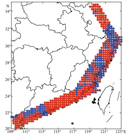
Fig.8 The stations that the difference of extreme wind speed between simplified and non-simplified track models can be explained (red dots) and not be explained(blue dots) by the difference of typhoon minimum approach distance or central pressure difference

In Test 1, the empirical distribution is adopted.Taking Test 1 as the controlled trial, the numerical experiments adopting the Weibull distribution,Gumbel distribution, and GPD are defined as Test 4,Test 5, and Test 6, respectively. The specific settings for Tests 1 and 4-6 are listed in Table 3.

Figure 9 shows the estimated V50in Test 4 (Fig.9a)and the wind speed difference between Tests 4 and 1(Fig.9b). It can be seen from Fig.9b that in most areas of China’s southeast coasts, the wind speed predicted by the Weibull distribution is lower than predicted by the empirical distribution, especially in Fujian and Guangdong provinces. The MD of the predicted wind speed is about -5.5 m/s and the MRD is about 11.3%.For the estimated V100, the MD is about -6.8 m/s and the MRD is about 13.0%.

Figure 10 shows the estimated V50in Test 5(Fig.10a) and the wind speed difference between Tests 5 and 1 (Fig.10b). Figure 10b indicates that over the entire southeast coastal region of China, the wind speed predicted by the Gumbel distribution is higher than that predicted by the empirical distribution,especially in Guangdong Province. The MD of the predicted wind speed is about 7.3 m/s and the MRD is about 19.5%. These values become 10.3 and 23%,respectively, for V100.

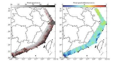
Fig.9 Maps of extreme wind speed (m/s) for 50-year return period in Test 4 (a) and the wind speed difference (m/s) between Tests 4 and 1 (b)

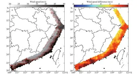
Fig.10 Maps of extreme wind speed (m/s) for 50-year return period in Test 5 (a) and the wind speed difference (m/s) between Tests 5 and 1 (b)

Figure 11 shows the estimated V50in Test 6(Fig.11a) and the wind speed difference between Tests 6 and 1 (Fig.11b). Figure 11b shows that over the entire southeast coastal region of China, the wind speed predicted by the GPD is lower than that predicted by the empirical distribution, especially in Fujian and Guangdong provinces. The MD of the predicted wind speed is about -8.5 m/s and the MRD is about 17.3%. For the estimated V100, the MD is about -8.8 m/s and the MRD is about 17.3%.

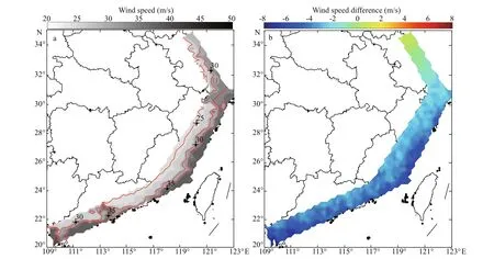
Fig.11 Maps of extreme wind speed (m/s) for 50-year return period in Test 6 (a) and the wind speed difference (m/s) between Tests 6 and 1 (b)

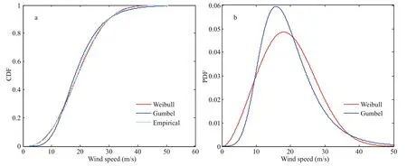
Fig.12 Cumulative probability curve (a) and probability density curve (b) of diff erent extreme value models for one example station

From the above analysis, it can be seen that the wind speed predicted by diff erent extreme value models is GDP ＜ Weibull ＜ Empirical＜ Gumbel. We analyze the extreme value distribution function itself to explain this phenomenon. Taking the extreme wind speed sequence of one station as the sample, we fit the parameters of four extreme value distributions and get their cumulative probability curve (CDF) and probability density curve (PDF), as shown in Fig.12.Since GDP is for the sample with wind speed exceeding the threshold, it is impossible to compare it with other extreme value models. It can be seen from Fig.12a that at the end of the CDF, which is decisive for predicting extreme wind speed, the cumulative probability is Weibull ＜ Empirical ＜ Gumbel, that is to say, for the same return period, the extreme wind speed is Weibull ＜ Empirical ＜ Gumbel. It can also be seen from Fig.12b that at the right tail of the PDF, the tail of Gumbel distribution is longer than that of Weibull distribution, so the predicted extreme wind speed is also larger. For GDP, the shape parameter is less than 0, which belongs to short-tailed distribution,so the predicted extreme wind speed is smaller. The extreme value distributions for other research stations are similar with those of the example station.

4 ESTIMATION ON RETURN PERIOD OF TYPHOON WIND SPEED

Based on the generated 1 000-year virtual typhoons for Northwest Pacific basin, we can predict the extreme wind speed of diff erent return periods at a certain site, which can provide reference for the design of critical structures and typhoon disaster mitigation. Conversely, given a typhoon event, we can calculate the return period of the maximum wind speed caused by the typhoon at a certain site to assess its risk. In this study, we select Test 1 to estimate the return period of typhoon wind speed. This is because,from Section 3.1, we can know the correlation in the decay model of Vickery and Twisdale (1995b) is better than that of Vickery (2005) for most regions. In simplified empirical track model, some secondary explanatory variables are eliminated which makes it simpler and more practical. Referring to Li and Hong(2014, 2016), Hong et al. (2016) and Chen and Duan(2018), the empirical distribution is used and it should be preferred when the sample size of wind speed is large.

The strongest typhoons aff ecting China coasts in the past four years are Meranti (2016), Hato (2017),Mangkhut (2018), Lekima (2019), and the tracks of the four typhoons are shown in the Fig.2. The return periods of the maximum wind speeds (representing 10-min mean wind speed at 10-m height) at diff erent sites caused by these four typhoons are calculated.Firstly, the typhoons aff ecting a certain site (typhoons passing within 250 km of the site) are abstracted from the 1 000-year virtual typhoons generated by simplified empirical track model in the Northwest Pacific basin. Secondly, the maximum wind speeds of these typhoons are calculated by using YM wind field model to form the extreme wind speed series vi( i=1,2, ∙∙∙, m). Thirdly, the YM model is used to simulate the observed typhoon and calculate the maximum wind speed v at the same site. Fourthly, judge the rank i of v in the extreme wind speed series. Finally, the return period is calculated by the following formula:

where λ is the typhoon annual occurrence rate at a certain site, m is sample size.

We first calculate the return periods of the maximum wind speeds of typhoons Meranti (2016),Hato (2017) and Lekima (2019) at 579 sites (black asterisks in Fig.2). The results are shown in the Fig.13.It can be seen that the return period of maximum wind speed at diff erent sites caused by diff erent typhoons only changes significantly near the typhoon landing points. The return period decreases rapidly with the increase of distance from landing point.

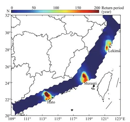
Fig.13 Maps of return periods (years) of maximum wind speeds for typhoons Meranti, Hato, and Lekima at 579 sites

In order to further reflect the variation of return period with diff erent sites, we select 26 stations along the China’s coasts, numbered 19-44 in Fig.2 and calculate the return periods of the maximum wind speeds caused by the four typhoons at these stations.The results are shown in the Fig.14. It can be seen that typhoon Meranti produced the extreme wind speed of 200-year return period at station 33 and Lekima produced the extreme wind speed of 110-year return period at station 28. Hato (2017) and Mankhut (2018)have similar landing point and produced the extreme wind speed once in a century at station 39. The return period of the station adjacent to the station with the maximum return period (distance of 100 km) is still considerable, and that of the station further away(distance of more than 200 km) decreases rapidly to 1.Due to the northward movement of typhoon Lekima,a considerable return period is also generated at stations 19-21. In addition, we can see that the stations with the second largest return period are all located on the right side of the typhoon track,indicating that the right side of typhoon is indeed more dangerous.

We also analyze the sensitivity of the return periods of the four typhoons at 26 stations to diff erent typhoon track models, decay models, and extreme value distributions. We compare the return periods of four typhoons at 26 stations under the simplified and nonsimplified typhoon track models as shown in Fig.15 and find the return periods predicted by the nonsimplified track model for most stations are relatively large. We calculate the mean minimum approach distance and central pressure difference when typhoons are closest to the coastal station based on the virtual typhoon events obtained by the two track models. It is found that for most stations, the minimum approach distance of the non-simplified model is larger than the result of the simplified model.Therefore, the extreme wind speed series are smaller,and the predicted return period is larger. At station 33,the pressure difference of the non-simplified model is greater than that of the simplified model, so the predicted return period is relatively small.

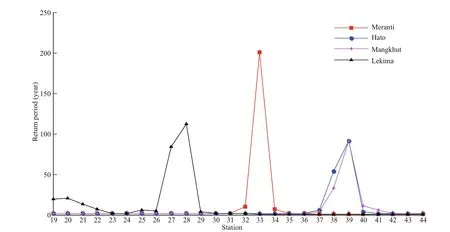
Fig.14 Return periods of maximum wind speeds for typhoons Meranti, Hato, Mangkhut, and Lekima at 19–44 coastal stations

Figure 16 shows a comparison of the return periods of four typhoons at 26 stations when Vickery and Twisdale (1995b) and Vickery (2005) decay models are used. It can be seen that the difference of return period between the two decay models is very small.Based on the analysis in Section 3.1, this is mainly due to the small difference of the decay pressure difference between the two models after typhoon landing.

Figure 17 shows a comparison of the return periods of four typhoons predicted by diff erent extremum distributions at 26 stations. It can be seen that for most stations, the return period predicted by diff erent extreme value distributions is: GDP ＞ Weibull ＞Empirical ＞ Gumbel, which has been analyzed in Section 3.3.

Fig.16 Comparison of the return periods of four typhoons at 19–44 coastal stations between Vickery and Twisdale (1995b)and Vickery (2005) decay models

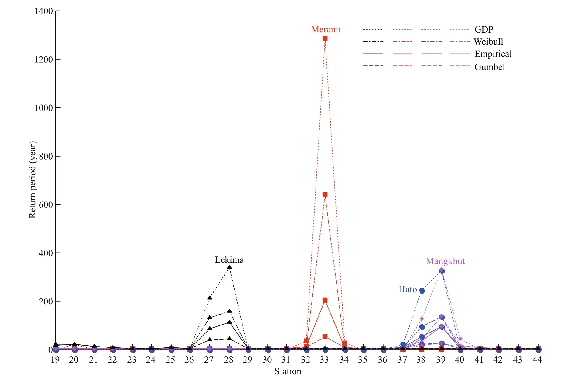
Fig.17 Comparison of the return periods of four typhoons predicted by diff erent extremum distributions at 19–44 coastal stations

Finally, we calculate the return periods of the maximum wind speeds generated by four typhoons at their landing point under the six groups of tests in Table 3, respectively. The results are shown in the Table 4. Because some landing points are close to the center of typhoon, the wind speed is not very large, so the return period is relatively small. We have analyzed the reasons for the differences of return periods in diff erent tests in Sections 3 and 4, which will not be discussed here.

Table 4 Return periods of the maximum wind speed generated by typhoons Meranti, Hato, Mangkhut, and Lekima at their landing point

5 CONCLUSION

In this paper, we described a technique for analyzing typhoon risk based on the empirical track model. We quantitatively investigate the sensitivity of the typhoon wind hazard model to diff erent typhoon decay models, the simplified and non-simplified typhoon tracking models, and diff erent extreme value distributions. We found the diff erent typhoon decay models have least influence on the predicted extreme wind speed, and the MRD from the control group is only about 3%. The predicted wind speed by the nonsimplified typhoon-tracking model is larger than that from the simplified tracking model in the coastal regions of northern Guangdong and Fujian provinces.The MRD of predicted V50is about 9.8%. Throughout the southeast coast of China, the predicted wind speed from the Weibull (GPD) distribution is lower than that from the empirical distribution and the MRD of the V50is about 11.3% (17.3%). The predicted wind speed from the Gumbel distribution is higher than that from the empirical distribution and the MRD for V50is up to 19.5%. We selected four super typhoons Meranti(2016), Hato (2017), Mangkhut (2018), Lekima(2019), and estimated the return periods of typhoon wind speeds along the China southeast coast in order to assess their risk. We found the return period decreases rapidly with the increase of distance from typhoon landing point.

6 DATA AVAILABILITY STATEMENT

The observed typhoon data that support the findings of this study are available in the CMA-repository(http://tcdata.typhoon.org.cn). The datasets generated during the current study are available from the corresponding author on reasonable request.

7 ACKNOWLEDGMENT

Data from the CMA-STI Best Track Dataset for Tropical Cyclones over the Western North Pacific online dataset are gratefully acknowledged. Thanks are extended to reviewers.