The evapotranspiration and environmental controls of typical underlying surfaces on the Qinghai-Tibetan Plateau

JinLei Chen,Jun Wen,ShiChang Kang,3,XianHong Meng,XianYu Yang

1. State Key Laboratory of Cryospheric Science, Northwest Institute of Eco-Environment and Resources, Chinese Academy of Sciences,Lanzhou,Gansu 730000,China

2. Key Laboratory of Land Surface Processes and Climate Change, Northwest Institute of Eco-Environment and Resources,Chinese Academy of Sciences,Lanzhou,Gansu 730000,China

3.CAS Centre for Excellence in Tibetan Plateau Earth Sciences,Beijing 100101,China

4.College of Atmospheric Sciences,Chengdu University of Information Technology,Chengdu,Sichuan 610225,China

ABSTRACT To reveal the characteristics of evapotranspiration and environmental control factors of typical underlying surfaces (alpine wetland and alpine meadow)on the Qinghai-Tibetan Plateau,a comprehensive study was performed via in situ observations and remote sensing data in the growing season and non-growing season. Evapotranspiration was positively correlated with precipitation, the decoupling coefficient, and the enhanced vegetation index, but was energy-limited and mainly controlled by the vapor pressure deficit and solar radiation at an annual scale and growing season scale, respectively. Compared with the non-growing season, monthly evapotranspiration, equilibrium evaporation, and decoupling coefficient were greater in the growing season due to lower vegetation resistance and considerable precipitation. However, these factors were restricted in the alpine meadow. The decoupling factor was more sensitive to changes of conductance in the alpine wetland.This study is of great significance for understanding hydro-meteorological processes on the Qinghai-Tibetan Plateau.

Keywords:evapotranspiration;control factor;typical underlying surfaces;Qinghai-Tibetan Plateau

1 Introduction

Evapotranspiration (ET) is a crucial factor in terrestrial hydrological and ecological processes (Chenet al., 2014). It affects climate change through soil moisture, water budgets, vegetation productivity, and carbon cycle (Junget al., 2010). Besides, it is also one of the crucial linkages that represent the interaction between the atmosphere and land surface (Panet al., 2020). Therefore, studyingETis essential for elucidating local hydro-meteorological processes and their links with other land surface processes.The Qinghai-Tibetan Plateau (QTP) is known as Asia's water tower. It is very sensitive to global climate changes and has great impacts on the weather and climate of China due to dynamic and thermal effects (Immerzeelet al.,2010).In recent years,warming of the QTP was approximate twice the global average (You et al.,2016), and it promoted the release of sensible heat and latent heat(ETis the main component)and affected the climate evolution in China,Asia and the world(Yuet al.,2011).

In recent decades, the mechanisms ofETand its environmental factors have been studied. A series of significant conclusions have been made using micrometeorological measurements, parameters, and models on various underlying surfaces, such as alpine and grazing steppes (Liet al., 2006; Maet al., 2015),grasslands (Weveret al., 2002; Yueet al., 2018;Zhanget al., 2019), trees, forests (Takanashiet al.,2010; Zhuet al., 2014; Chenet al., 2018), shrublands(Jiaet al.,2016),croplands(Dinget al.,2013;Sutherlinet al., 2019), and mixed plantations (Tonget al.,2017). However, the applicability of these findings is limited to the QTP, whereETis different due to unique topographical and landscape features (Guet al., 2008). With increasing ground temperature (Liu and Chen, 2000), assessments for different ecosystems on the QTP can better understand the hydrologic processes as well as regional climate changes.However, the characteristics ofETand its environmental factors over vulnerable alpine land surfaces on the QTP,especially alpine wetland (AW) and alpine meadow(AM), were rarely discussed in previous studies.Therefore, comprehensive studies with a combination of in situ observations and satellite products are essential to better understand the land-atmosphere processes on the QTP.

Alpine meadows and alpine wetlands are crucial underlying surfaces on the QTP which are sensitive to climate change. In this work, variations of hydrometeorological factors and their relationships are discussed with various hydro-meteorological indicators.In addition,ETand environmental factors of two typical underlying surfaces were investigated and compared with remote sensing data and in situ observations in the Maqu alpine meadow and the Zoige alpine wetland to reveal the characteristic ofETprocesses and the function of environment control factors on the QTP. This paper is structured as follows.The second part is the introduction of the study area and datasets. The third section includes the methodology. The fourth part is analysis and discussion for the results. The last section is the conclusions of this study.

2 Study area and datasets

Maqu and Zoige are typical alpine meadow and alpine wetland environments on the QTP, respectively, influenced by the East Asian monsoon climate. They experience a cold and moist environment and have long frost periods and large temperature differences between day and night (Chenet al.,2020). The altitude varies from 3,600 m to 3,800 m above sea level, and the average annual temperatures are 2°C (Maqu)and 0.7°C(Zoige), respectively. The mean annual value of total precipitation is 505 mm in Maqu(Chenet al.,2016),and 600-800 mm in Zoige (86% of the rainfall occurs from late April to October).

Rsis solar shortwave radiation,LErepresents latent heat flux,His sensible heat flux,βrepresents the Bowen ratio,PandTare atmospheric pressure and air temperature, respectively.rh0represents specific humidity,Precis precipitation,ETis evapotranspiration,SMis soil moisture at 10 cm depth,Eeqis equilibrium evaporation,Eimis another part of evapotranspiration which is imposed by surrounding air, α is the Priestley-Taylor coefficient,VPDandLAIare vapor water pressure deficit and leaf area index,respectively.EVIis the enhanced vegetation index.rcandraare bulk vegetation resistance and aerodynamic resistance, respectively. Ω is the decoupling coefficient.α,β,rc,ra, and Ω are the average of midday values(10:00-16:30).

As presented in Figure 1, two observation sites,Alpine Meadow (102°06'E,33°55'N) and Alpine Wetland (102°48'E, 33°54'N), were established and maintained for hydrological and ecological monitoring by the Zoige Plateau Wetland Ecosystem Research Station of the Chinese Academy of Sciences. Both sites had a set of eddy covariance systems, an ECH20 EC-TM, and a T-200 precipitation gauge produced by Campbell Scientific in Utah, USA.Downward shortwave radiation, downward longwave radiation, upward shortwave radiation, upward longwave radiation, sensible and latent heat fluxes,precipitation, wind speed, friction velocity, atmospheric pressure, specific humidity, air temperature,air density, soil temperature, soil moisture, and soil heat flux at 5 cm and 10 cm depths were measured at every 30 min and collected by a CR5000 data acquisition unit.Datasets from 2016-2017 were used after quality control, and mean energy budgets and environmental factors(presented in Table 1)were calculated for growing season (May-September), nongrowing season (October-April), and year-round,for which the Priestley-Taylor coefficient (α), Bowen ratio (β), vegetation resistance (rc), aerodynamic resistance (ra), and decoupling coefficient (Ω) are midday (10:00-16:30) averages. The enhanced vegetation index (EVI,16 days mean value composited by the spatial resolution of 250 m) and leaf area index(LAI, eight days mean value composited by the spatial resolution of 500 m) obtained from the Moderate Resolution Imaging Spectrometer were used to estimate plant growth (https://ladsweb.modaps.eosdis.nasa.gov/search/).

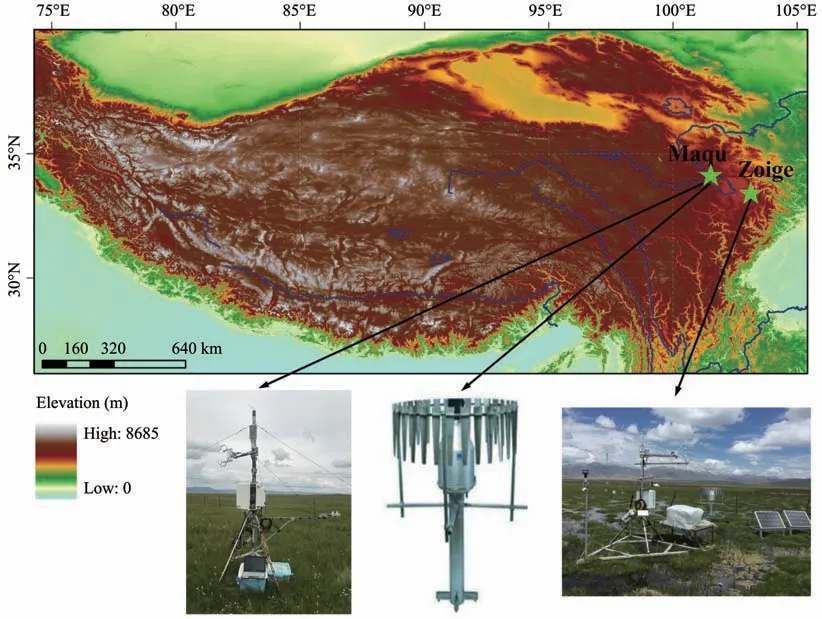
Figure 1 The geographic location of the observation sites

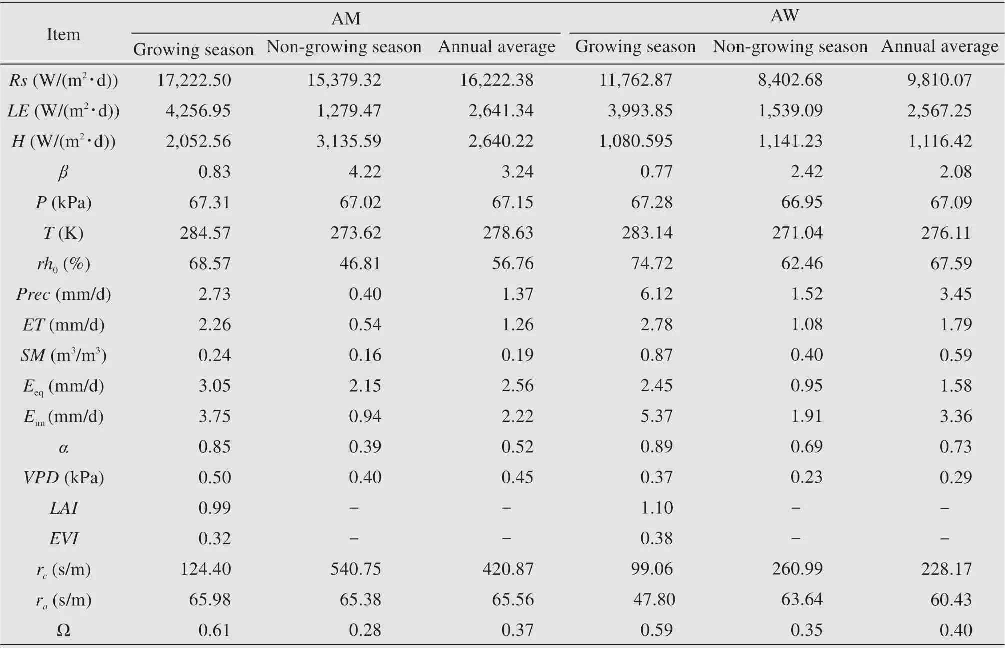
Table 1 Statistics of energy budgets and hydro-meteorological factors of AM and AW in the growing season and non-growing season

3 Methodology

According to the theory of Penman-Monteith(Monteith, 1965; Monteith and Unsworth, 2013), the vegetation conductance (gc, m/s) and vegetation resistance(rc,s/m)can be estimated as follows:

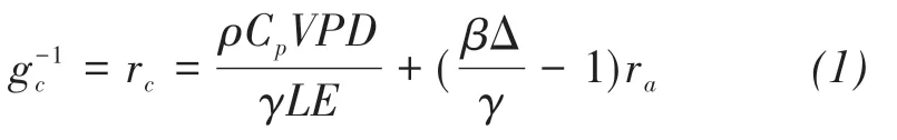
whereρand Δ are air density (kg/m3) and slope of the saturation vapor pressure curve (kPa/°C), respectively;Cp=1.013×103J/(kg·℃)is specific heat capacity of the air;γ(psychometric constant,kPa/°C)(Donatelliet al., 2006), andVPDandracan be calculated as follows:

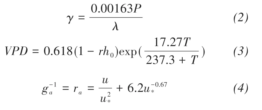
whereuandgarepresent wind speed (m/s) and aerodynamic conductance (m/s), respectively.u*is friction velocity,andλis the function of air temperatureT(°C)(Donatelliet al.,2006):

The decoupling coefficient indicates the relationship between the atmospheric boundary layer and the ecosystem surface (Jarvis and Mcnon-aughton, 1986);it is the weighting coefficient ofEeqandEimand varies from 0 to 1. When Ω=0,ETis controlled byVPDwhich means a full coupling between canopy surface and atmosphere in the boundary layer.When Ω=1,ETis controlled byRs, and the canopy surface is decoupled from the atmosphere.

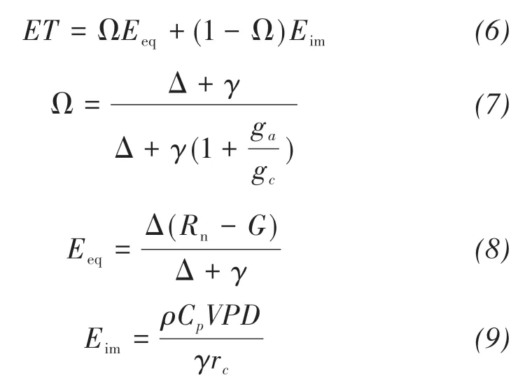
in whichEeqdepends on the available energy (i.e., solar radiation),andEimis the part ofETimposed by the surrounding air.Rnis net radiance (W/m2).Gpresents surface heat flux (W/m2) and can be obtained by the PlateCal method:

whereCvandGzare specific heat capacity of the soil(J/(m3·°C)) and soil heat flux at depthz(cm), respectively.Ts(z) represents soil temperature at corresponding depth, in which surface temperatureT0obeys the Stefan-Boltzmann law:

whereL↑andL↓are upward longwave radiation and downward longwave radiation, respectively. The specific radianceε=0.97, and the Stefan-Boltzmann constant isσ=5.6704×10-8W/(K4·m2). The ratio betweenETandEeqis the Priestley-Taylor coefficient(α),which can be used to assume a closed volume and constant net radiation over a wet ecosystem (Mcnonaughton and Spriggs,1986):

4 Results and discussion

4.1 Hydrological factors and bulk parameters

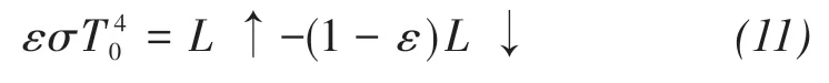
The monthly cumulative precipitation,ET, and monthly mean soil moisture in AM and AW were calculated and presented in Figures 2a and 2c,respectively.ETwas strongly correlated with precipitation(Prec,R2=0.83) in AM, while a relatively low correlation(R2=0.53)was shown in AW.Affected by the summer monsoon, precipitation was mainly concentrated from May to September(longer in AW).The poor correlation was attributed to excessive precipitation with limited conditions forET. The surplus rainfall ran off and drained into rivers or penetrated into the deep soil, which can be corroborated by the near-saturated soil moisture at 10 cm depth. Precipitation,ET, and soil moisture (SM) were greater in AW than that in AM during the growing season when SM was renewed by monsoon rainfall.The low valley in August was generated by intense radiation. According to Equation(6),ETcan be decomposed to a function ofEeqandEim, with a weighting coefficient of the decoupling factor. Monthly cumulativeEeqandEim, and monthly mean decoupling factor are displayed in Figures 2b and 2d, in which all maximum values at both sites occurred in summer.Eeqwas controlled by the available energy and temperature, and had larger values in AM than that in AW, whileEimshowed opposite tends.The decoupling factor represents the effects ofVPDandRsonETand controls the rates of canopy transpiration, which is high whenETwas mainly controlled byRsin the growing season and low whenVPDwas the dominating factor in winter.Ω had similar values at the two sites in the growing season, while it was larger in AW during the nongrowing season.

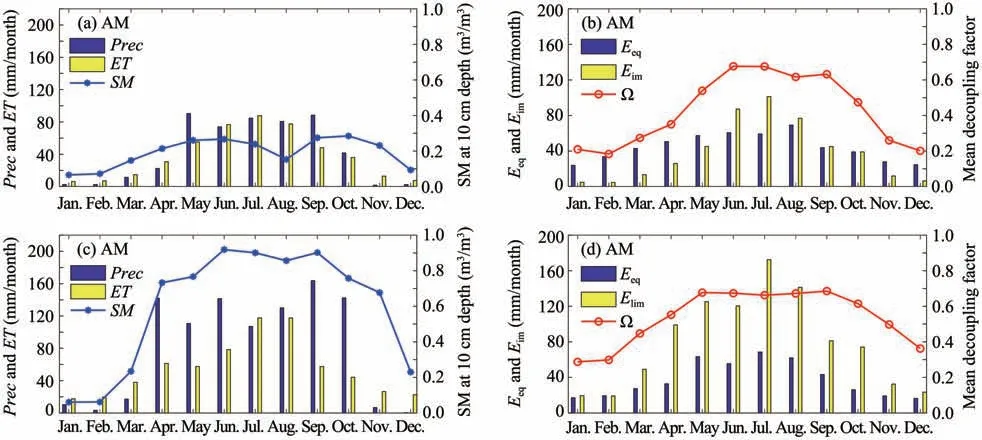
Figure 2 The variation of hydrological factors coupled to evapotranspiration

Theraandrcindicate the outside part's energy transfer conditions (between the reference height and the active canopy surface) and inside part (between the interior and exterior of leaves), respectively. The monthly mean midday variations are presented in Figures 3a-3b. Their average values were higher in AM during the growing season and non-growing season, as well as annually (Table 1). Compared with the single underlying landscape in AM, AW is covered by mixed water and meadows, making the monthlyralower (except in the winter, when the ice surface increases the resistance) than that in AM.Therchad low values in both AM and AW during the growing season, while the increase was greater in AM during the non-growing season. The monthly mean midday variations inαandβare presented in Figures 3c-3d. Theαwas consistently lower than one in AM and AW, which means that the water supply was restricted and significantly affectsET. The water limitation was more severe in the non-growing season,especially in AM.Latent heat flux was dominant in the growing season due to abundant precipitation and favorable surface conditions. In contrast,sensible heat flux was higher in the non-growing season when its distribution was more than twice in AM than that in AW.

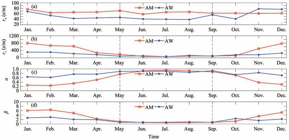
Figure 3 Variations in monthly average midday(a)aerodynamic resistance(ra),(b)vegetation resistance(rc),(c)Priestley-Taylor coefficient(α),and Bowen ratio(β)

4.2 Decoupling factor

Figure 4 shows the frequency of the decoupling factor counted with an interval step of 0.05 and the corresponding meanETat midday.The proportions of Ω below 0.5 were 64.85% and 67.55% in AM and AW, respectively, which implies thatETprocesses were mainly coupled toVPDat two sites on an annual scale. However, the average in Table 1 shows that evaporation was controlled primarily by solar radiation during the growing season. The frequency distribution had two peaks in AM. One occurred when Ω∈(0.05, 0.1], and the other happened when Ω∈(0.6,0.65]. The first peak was dominant, and Ω at (0.05,0.35] occupied over half of the total. AW had only one peak,which was shown at(0.40,0.45].The correspondingETincreased with increasing Ω within (0,0.9] at both sites. However, an obvious decrease occurred at (0.9, 0.95]. Further study is needed to explain this phenomenon, although one possible explanation is water limitation at midday (Karamet al.,2007),which has yet to be verified.

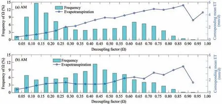
Figure 4 Frequency distribution of Ω and corresponding ET at midday

ETis directly determined by the ground surface conductance, which is made up of vegetation conductance and aerodynamic conductance. The variations ofgaandgccompared with decoupling factors in AM and AW are presented in Figure 5, in which conductance was the average within each interval of 0.005 m/s and Ω was the mean at the corresponding times. It is clear thatgaandgcresponded in opposite trends to environmental factors. Ω decreased and increased with increasinggaandgc, respectively. It was briefly dominated bygawhen the conductance was within 0.01 m/s in AM and within 0.015 m/s in AW,after which it was controlled bygc. The distribution of the decoupling factor was more compact in AW than AM.Ω was larger in the same interval ofgcand smaller in the same interval ofga. This finding means that Ω was more sensitive to the change in conductance in AW.

4.3 Vegetation parameters

Normalized difference vegetation index was often used to modulate the energy partition (Yueet al.,2018). However, it is easy to reach saturation in the flourishing period of vegetation growth.EVIcan overcome this weakness and truly reflect vegetative growth and change processes.Figure 6 displays the relationships betweenEVIandETin AM and AW, in whichETwas the cumulative value in eachEVIcycle(16 days).EVIvaried with the change in vegetation from 0.22 to 0.39 in AM and from 0.21 to 0.47 in AW.The corresponding averages ofEVIfor AM and AW were 0.31 and 0.35, respectively. Strong correlations betweenETandEVI(R2=0.81 and 0.73) were observed in AM and AW.ETincreased with increasingEVI, and it was more significant in AM, which was fully covered by vegetation. In addition,ETwas discrete for the nonhomogeneous distribution of meadows and water in AW.

Thegcis strongly correlated with environmental and biological factors,includingVPDandLAI(Weveret al., 2002). Figure 7 shows the relationships between middaygcandLAI(a and c)/VPD(b and d) in AM and AW.gcandVPDwere the mean values for oneLAIcycle (eight days), after whichLAIandVPDwere averaged at an interval of 0.1 andgcwas expressed as the mean at corresponding times to reduce observation errors.LAIwas larger in the growing season at both sites, while the averageLAIwas larger in AW (Table 1).gcincreased with increasingLAIat both sites.Compared to that of AW, the response rate was larger in AM during the non-growing season, while it was smaller in the growing season.The latent heat flux was affected byVPDthroughgc.VPDwas low in AW due to abundant water supply. Generally,gcdecreased with the increasing ofVPDin AM and AW, and was higher in the growing season at the sameVPD.

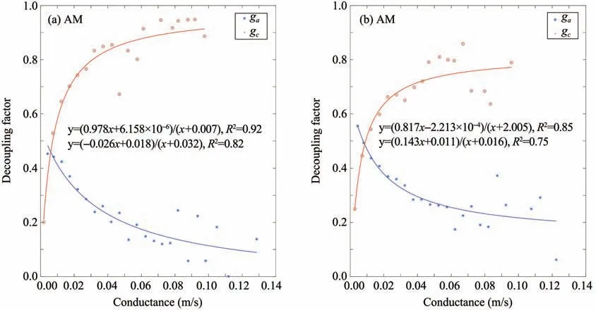
Figure 5 Variations of Ω versus aerodynamic conductance(ga)and vegetation conductance(gc)in AM and AW,respectively

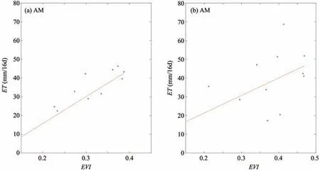
Figure 6 Relationships between EVI and ET in the growing season

5 Conclusions

This research comprehensively studied the characteristics ofETand its environmental factors for typical underlying surfaces via in situ observations and remote sensing data.The findings have great significance for understanding the energy and water transfer processes among land, vegetation, and atmosphere and contributes to the protection of water resources in alpine wetland and alpine meadow on the Qinghai-Tibetan Plateau. The following are the main results.

(1)ETwas positively correlated with precipitation,EVI, and decoupling factor for both typical underlying surfaces, especially in AM, and was energylimited and caused by vapor water pressure deficit and solar radiation at annual scale and growing season scale,respectively.

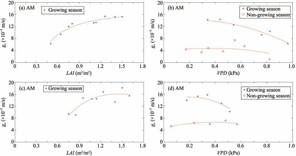
Figure 7 Relationships between vegetation conductance and(a and c)LAI and(b and d)VPD in the growingseason and non-growing season

(2) The coupling between land and atmosphere was higher in AW than AM during the non-growing season. However, the difference is small in the growing season. The decoupling factor was more sensitive to changes of conductance in AW.

(3) Bulk vegetation resistance and aerodynamic resistance were greater in AM, and aerodynamic resistance rapidly increased during the non-growing season.Water supply was restricted,and the limitation was more severe in the non-growing season,especially in AM.

(4) Vegetation conductance was negatively correlated with vapor water pressure deficit with higher values in the growing season.

Acknowledgments:

This work is financially supported by the National Natural Science Foundation of China (Grant Nos.42005075 and 41530529), the Second Tibetan Plateau Scientific Expedition and Research Program (STEP)(No. 2019QZKK0605), the State Key Laboratory of Cryospheric Science(Grant Nos.SKLCS-ZZ-2020 and SKLCS-ZZ-2021) and Foundation for Excellent Youth Scholars of "Northwest Institute of Eco-Environment and Resources", CAS (Grant No. FEYS2019020). The authors declare no competing interest in this paper.Our cordial gratitude should be extended to anonymous reviewers and the Editors for their professional and pertinent comments on this manuscript.