Enhanced two-loop model predictive control design for linear uncertain systems

Mohammad-Ghassem FARAJZADEH-DEVIN and Seyed Kamal HOSSEINI SANI

Department of Electrical Engineering, Ferdowsi University of Mashhad, Mashhad 1696700, Iran

Abstract: Model predictive controllers (MPC) with the two-loop scheme are successful approaches practically and can be classified into two main categories, tube-based MPC and MPCbased reference governors (RG). In this paper, an enhanced twoloop MPC design is proposed for a pre-stabilized system with the bounded uncertainty subject to the input and state constraints. The proposed method offers less conservatism than the tube-based MPC methods by enlarging the restricted input constraint. Contrary to the MPC-based RGs, the investigated method improves tracking performance of the pre-stabilized system while satisfying the constraints. Additionally, the robust global asymptotic stability of the closed-loop system is guaranteed in a novel procedure with terminal constraint relaxation. Simulation of the proposed method on a servo system shows its effectiveness in comparison to the others.

Keywords: model predictive control (MPC), robust control, cascade control, constraint satisfaction.

1. Introduction

In the past decade, model predictive control (MPC) has had an explosive growth of use in the industry due to its great success in controlling multivariable systems and its ability to handle complex systems with hard control constraints [1]. MPC methods usually employ an online finite optimization problem to calculate the control signal.Although there is a great interest for utilizing MPC in fast applications such as aerospace, automotive or mechatronics, the computational cost of MPC and its sensitivity to the model as well as uncertainties are the main obstacles[2].

The computational burden of MPC increases exponentially when the system uncertainty is involved in the MPC problem. It is mainly due to the necessity of solving a closed-loop MPC problem, which means that the decision variable of the optimization problem should be considered as a sequence of control laws but not a sequence of control actions [3].

Among the literature, several methods are developed to simplify the required calculation of the closed-loop (robust) MPC by employing two control loops, where usually the MPC is located in the outer-loop and an ancillary control is placed in the inner-loop such as tube-based MPC (TB-MPC) methods and MPC-based reference governors (RG).

TB-MPC methods [4–9] are developed in order to simplify the required online calculation. These methods utilize a nominal MPC in the outer-loop and a local feedback (ancillary) controller in the inner-loop. Their objective is to maintain all possible trajectories of the uncertain system inside a sequence of admissible regions called reachability tube [10] by the ancillary controller. The tube can be calculated online or approximated offline. However,the online exact calculation is usually computationally difficult [11] and offline approximation entails a high degree of conservatism [12].

MPC-based RGs [13–18] concentrate on pre-stabilized(closed-loop) systems which have proper tracking performance (and robustness). Then, adding an MPC to the system (in the outer-loop) to enforce the state and control constraints to the pre-stabilized system by modifying the reference, whenever necessary [19]. Although, special versions of MPC-based RGs guarantee the robustness of the closed-loop system in presence of bounded uncertainty [13,16,17], improving the tracking performance is not covered in these methods.

There exist some other custom-designed MPC methods with the two-loop scheme [20–25]. These methods usually handle the system’s uncertainty and/or nonlinearity in the inner-loop and satisfy the constraint by the outer MPC loop. They are popular methods in fast applications especially in robotics for high robustness and simplicity of the calculation. However, they usually suffer from the casedependent design algorithm.

In this paper, we focus on a pre-stabilized linear time invariant system with bounded uncertainties, e.g., state estimation error, modelling error, disturbance, etc., and propose an enhanced two-loop MPC (TL-MPC) design to satisfy the input and state constraints, improve the closedloop tracking performance and guarantee the robust stability of the system. The proposed method uses two control loops sequentially, the inner-loop which is assumed to be pre-stabilized and the MPC loop which is responsible for the tracking performance improvement of the pre-stabilized system, satisfying the input and state constraints simultaneously. The proposed method is less conservative than the TB-MPC and improves the tracking performance of the pre-stabilized system contrary to the MPC-based RGs. The robust global asymptotic stability for the proposed method is guaranteed without the terminal constraint definition which leads to design complexity reduction in practice. Additionally, the open-loop model of the system is not required, and merely, an approximation of the closed-loop model is used instead.Consequently, the proposed method can be used for available closed-loop industrial systems to upgrade them and improve their performance without removing the existent controllers and thus with less design and computational cost.

In the following, Section 2 introduces the preliminaries and states the problem. Section 3 presents the proposed TL-MPC structure and its features. In Section 4, two examples are illustrated to compare the performance of the proposed method with nominal MPC [26] and TB-MPC[4]. Finally, concluding remarks are presented in Section 5.

2. Preliminaries and problem statement

Consider a discrete-time linear uncertain system in the form

where the vector x is the current system state, x+is the successor system state, u is the control input and w is the bounded disturbance. The matrices A ∈Rn×nandB ∈Rn×mare the state space matrices of (1) and D ∈Rn×nis a diagonal scaling matrix, where R denotes the set of real numbers.

Note that D is a scaling matrix and the dynamical model of the uncertainty is assumed to be unknown. Additionally, as it is presented in [27], w may contain the state estimation error, the structural uncertainty and the disturbance in general. The convex sets X ⊆Rnand U ⊆Rmare the hard state and input constraints, and the convex set W ⊂Rncontains the origin. The ancillary control loop(inner-loop) is employed by using a controller µ:Rn×Rm→Rmthat is determined in (2), where v ∈Rmis the input of the ancillary closed-loop system (3).

It is assumed that the states of the closed-loop system(3) can be estimated by the states of an approximated system (4), where the state vector z is the approximation of the state vector x, and the matrices Aaand Baare the approximation of the matrices Acland Bcl.

where Aa= Acl+∆A, and Ba=Bcl+∆B.

The vector of the model tracking error is defined as (5)and its dynamic is presented in (6), where g is the error dynamic function.

The following definitions are about robust stability properties of a discrete dynamical system G subject to bounded disturbance w, which are inspired from [7,26],where the tube Skis considered as a time varying set.

Definition 1Robust positive invariant A tube Sk⊆Rnis robustly positive invariant (RPI) for the system G, if ∀ xk0∈Sk, it holds that xk∈Skfor all wk∈W and for each k ＞k0∈N+, where N+is the set of natural numbers plus zero.

Let the Euclidean norm of a vector be denoted by |·| ,the distance between a vector v ∈Rnand any compact set S ⊆Rnbe defined byd} defines a set including S with the maximum distance dbetween any member of Bd,Sand compact set S, then we have the following definitions.

Definition 2Robust Lyapunov stability The closed RPI tube Sk⊆Rnis robustly Lyapunov stable for the system G, if for any ε ＞0 , there exists δ ＞0, such that for any initial condition xk0∈Bδ,Sk0a nd any disturbancewk∈W, which satisfies that xk∈Bε,Skfor all k ＞k0∈N+.

Definition 3Robust (global) asymptotic stability The closed RPI tube Sk⊆Rnis robustly and asymptotically stable for the system G with the region of attraction Ra⊆Rn, if it is robustly Lyapunov stable and|xk|Sk→0 as k →∞ for all xk0∈Raand ∀ wk∈W, ∀k ＞k0∈N+, and Ra=Rn.it is robustly globally asymptotically stable (RGAS) if

Assumption 1Giving a positive real number δ and a closed RPI tube Sk=Bδ,vk, then it is assumed that the tube Skfor the closed-loop system (3) is RGAS.

The idea of Assumption 1 was firstly introduced for robust RGs in [28], and additionally it had become popular in the robust MPC methods [19]. Assumption 1 is easily tractable since already there are a lot of robust linear control methods for this purpose and it is not necessary forδ to be small.

Remark 1Based on Assumption 1 and general results presented in [29], it is concluded that there exists a finite ε ∈R++, which is the maximum model tracking error, where R++denotes the set of positive real numbers.

Therefore, one has

or equivalently

The concepts of Assumption 1 and Remark 1 are better illustrated in Fig. 1. The input of the inner-loop v (·) is shown with the green curve, the closed RPI tube Skis defined as a ball around v(·) with radius δ and displayed with light green, the approximated state z(·) is shown with the blue curve and the real state x(·) with red, and their distance is always less than ε. Additionally, Assumption 1 implies that the distance between x(·) and Skasymptotically tends to zero over time. In other words, x falls into the tube Skultimately.

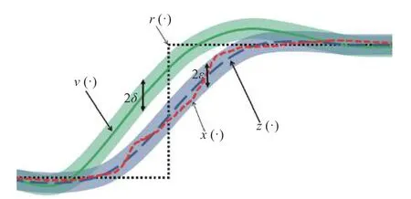
Fig. 1 Illustration of the concepts of Assumption 1 and Remark 1

3. The proposed TL-MPC

Consider the pre-stabilized system (3) with Assumption 1,then the proposed TL-MPC design is completed by utilizing the closed-loop system (3) as the inner-loop and adding a nominal model predictive controller based on the following optimization problem to improve the tracking performance of the closed-loop system (3) and satisfy the input and state constraints X and U. The TL-MPC optimization problem is

where N is the prediction horizon,is the minimum value of the cost function VN(·,·), v∗(·) is the optimal input sequence for the closed-loop system (3), and VN(·) is the set of feasible inputs for the optimal control problem PN(x0). The first element of the optimal sequenceis to the system (3) and the problem PN(·) is solved again at the next sample time. The cost function VN(·,·) is defined in (9).

where l(a,b)=aTQa+bTMb, ez=zr−z, ev=vr−v. The constraints are presented in (10)-(14).

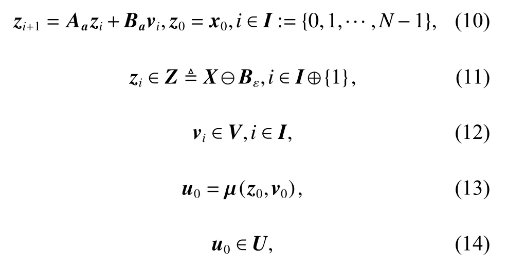
where the vectors zrand vrare the reference state and the reference input of the system (1), Q and M are weighting matrices, u0is the first input of the system (1), and Z and Vare feasible sets for the approximated state z and decision variable v respectively. The Minkowski set addition of two sets is indicated by ⊕, and the Minkowski difference is denoted by ⊖.

Iteratively, the first element of the optimization variableis applied to the ancillary loop (3) as the input(15). The TL-MPC design block diagram is investigated in Fig. 2 and the design procedure steps are summarized in Algorithm 1.

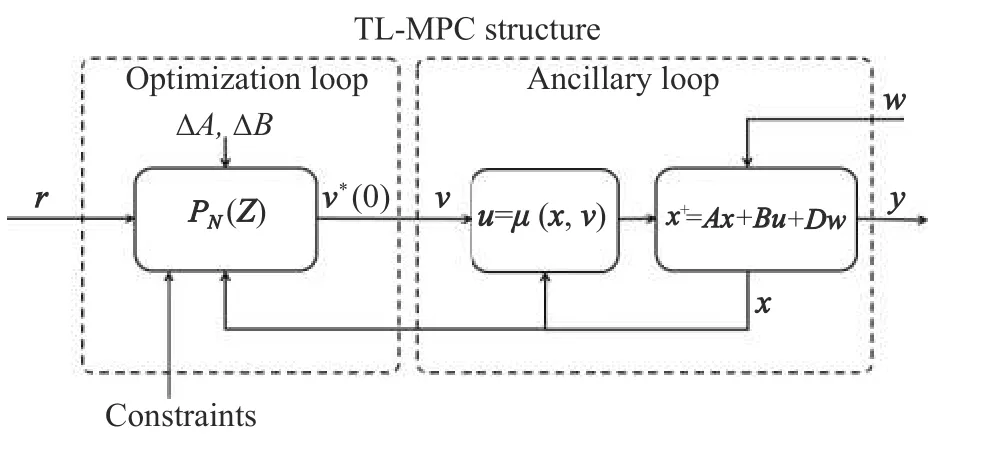
Fig. 2 TL-MPC design block diagram

Algorithm 1TL-MPC design steps

RequirementsThe approximated system model (4),control rule μ (2), the input and state constraints U and X,and the tracking error band ε (Remark 1).

Initializing:

Step 1Choose/calculate the reference state and the reference input vectors zrand vr.

Step 2Choose proper optimization parameters N, Q and M.

Step 3Calculate the restricted constraint Z (11) and new input constraint V (12).

Controlling:

Step 4Set the initial state of the optimization z0=x0.

Step 5Findby solving the optimization problem PN(x0) using the standard quadratic programming (QP)methods with the cost function (9) and constraints (10).

Step 6Applyto the inner-loop system (3) as the input according to (15).

Step 7Go to Step 4.

Remark 2The proposed TL-MPC design only needs to know the approximated values of the closed-loop matrices Aaand Ba, the control rule µ and the maximum of the error bound ε. Therefore, the value of the openloop model matrices A and B, the precise value of the closed-loop matrices Acland Bcl, as well as the error dynamics function g are not required to be known.

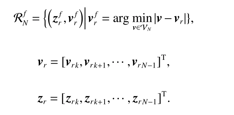
Robust global asymptotic stability of the proposed TLMPC design is guaranteed in Theorem 1 based on the set of feasible reference trajectorydefined as below.

Definition 4Given the set of feasible inputs VN, and the reference trajectory (zrk,vrk), then the set of feasible reference trajectoryis defined as

Theorem 1Robust global asymptotic stability of TLMPC Giving the set of feasible reference trajectorythe positive real value γ ∈R++, and the closed RPI tube Tk, thus

Then the proposed TL-MPC structure around the feasible reference trajectoryin the presence of unknown disturbance w ∈W is RGAS, i.e., the closed RPI tube Tkfor the system (15) is RGAS for all w ∈W.

ProofConsider an initial solution for the problem PN(·)as

then according to Assumption 1, the closed RPI tube Skfor the closed-loop system (3) is RGAS; also considering Remark 1, one has

which implies that the closed RPI tube S′kfor the approximated system (4) is RGAS, where

consequently,

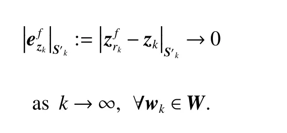
On the other hand, applying the optimal inputobtained by the optimization problem PN(x0) to the system(3) implies that

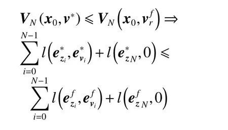
where

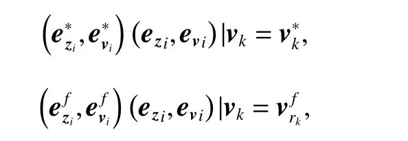
according to Definition 4, we have

which yields

For the approximated system (4), we have

then it is concluded that

which implies that

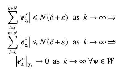
The proposed structure can facilitate the implementation of MPC, which is explained in the following remarks.

Remark 3In the proposed TL-MPC method, the initial state of the nominal system z0is recursively reset to the actual sate x0based on (10). This leads to the input constraint not to be restricted for the first control input u0presented in (14). Therefore, the investigated method offers less conservatism than the tube-based MPC methods.

4. Simulation results

Illustrative example 1In order to have a fair comparison, the proposed TL-MPC is compared with the TB-MPC[4] and the nominal MPC [26]. The example is similar to the illustrative example presented in Section 2 [26]. Suppose the system is described by x+=x+u with initial stateand the terminal cost isThe control constraint is u ∈[−1,1] and there are no state or terminal constraints. Suppose the prediction horizon N=2. Additionally, it is supposed that the reference signal r=3step(t −20) , where the function step(t)=1 if t ≥0,and step(t)=0t)=0 if t ＜0. The uncertain signal w(k)=w1(k)+d(k) , where w1(k) is a random signal belongs to [−0.2, 0.2] and d(k)=0.3step(t −30) is a disturbance signal. Fig. 3 shows the simulation result for the three control methods TL-MPC, TB-MPC and the nominal MPC, and Fig. 4 presents the control signals. A state feedback with K=−1, is considered for both TL-MPC and TB-MPC methods. In the first iterations (i ∈{0,1,···,4}) the tracking error is big and the control signals of the nominal MPC and TL-MPC are saturated (uMPC=uTL−MPC=−1), but TB-MPC is more conservative and uses fewer control signals. The reference is changed from 0 to 3 at i=20 and TL-MPC tracks the reference faster than the others. Despite of disturbance w1∈[±0.2] during all iterations, disturbance d is applied at i=30, where amplitude is 0 .3 and it continues until i =40. For the duration of i=30 to i=40, TL-MPC and TB-MPC show a better response than the nominal MPC in disturbance handling. This simulation implies that the proposed TLMPC structure is as robust as TB-MPC and as fast as the nominal MPC.

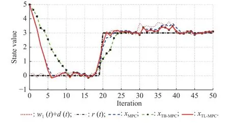
Fig. 3 Output of three different methods in illustrative example 1

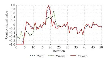
Fig. 4 Control signal of three different methods in illustrative example 1

Illustrative example 2Servo system The state space model of a DC motor is presented in (16)-(19),which is inspired from [30].

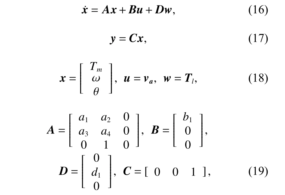
where x1is the torque of the motor, x2is the angular velocity of the motor and x3is the angular position of the motor. The motor parameters are determined in Table 1.The elements of the matrices A, B and D are as follows,Kie/Laand d1=−1/J. Then, the model can be simplified to (20)-(23).

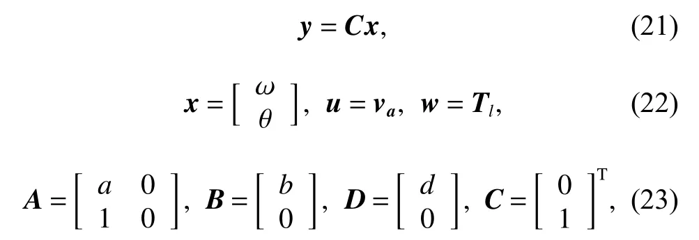
where a =−((Kie)2+FRa)/JRa, b =Kie/JRaandd=d1=−1/J . The block diagram of a DC servo system is shown in Fig. 5, where k1, k2are the servo controller gains andv is the reference input.

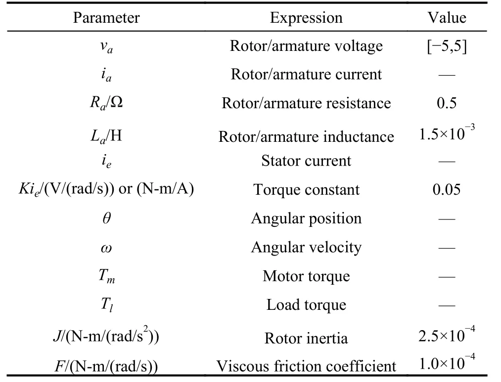
Table 1 Motor parameters

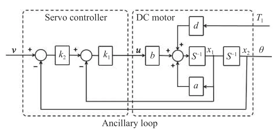
Fig. 5 Simple DC servo system block diagram

The control rule of the servo controller is as (24),where K= [−0.75 −65] and k=65. Thus, the closedloop system model is obtained as (25).

Suppose that the approximated model of the closedloop system is defined by Aa:= Acl+∆A and Ba:=Bcl+∆B, where ∆A:=10%Acland ∆B:=10%Bcl. It is measured practically that ε=[1, 0.006]T. By considering the sampling time ∆t=0.005 s, first order forward approximation ofis equal to (x+−x)/∆t, which is used to discretize the open loop, closed-loop and approximated systems. The uncertainty is supposed with two parts,Dw(t):=[w1(t)+d(t),0]Twhere w1(t) is a random signal that belongs to ± 3 rad/s , and the disturbance d(t) and the reference signal r (t) are considered as

The optimization control loop is added to the ancillary controller (24) by defining PN(z) as (7)-(14), where N=10, Z=R2, V=R, Q=[0 0;0 10] and M=0.1. The task of the optimization control loop is to improve the tracking performance of the servo system (25) and satisfy the input constraint u ∈U=[−5,5].

The reference and disturbance are applied to the DC motor model (20)-(23) with two different controllers individually: the servo controller (SC) (24), and the proposed TL-MPC. The angular position of the motor x2(t)is illustrated in Fig. 6, and Fig. 7 shows the rotor voltage of the motor u(t). Obviously, TL-MPC improves the tracking performance of the SC and satisfies the constraints with low conservatism.

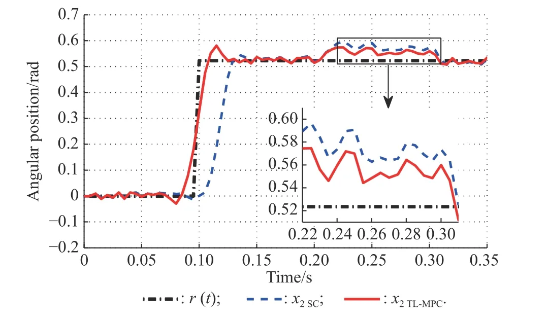
Fig. 6 Reference signal r(t) and the angular position x2(t) of the DC motor for the SC and the proposed TL-MPC in illustrative example 2

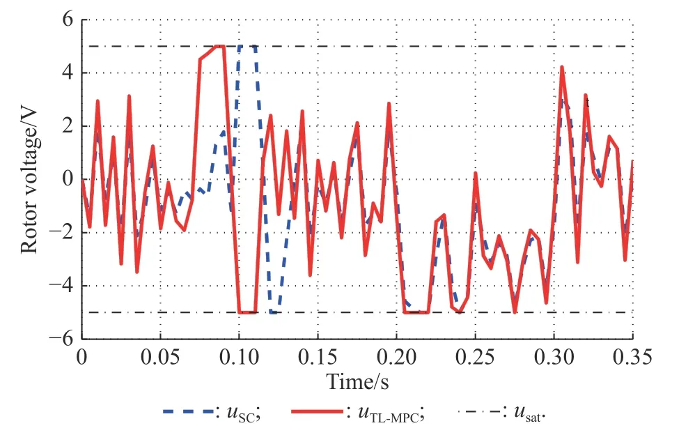
Fig. 7 Rotor voltage of the motor u(t) for the SC and the proposed TL-MPC

Numerical comparisonThe integral square error(ISE) and the ISE of the disturbance interval (ISE-DI) are used as performance indexes to show the superiority of the proposed algorithm than the others. The disturbance interval is i ∈{30, 31, ···, 40} for the illustrative example 1 and t ∈[0.2, 0.3] for the illustrative example 2.Table 2 shows that the proposed TL-MPC method has less ISE and ISE-DI than the other methods in both illustrative examples.

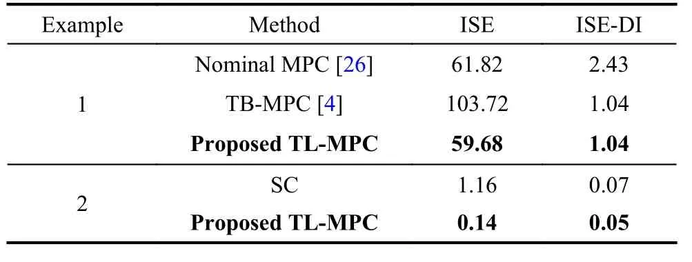
Table 2 Numerical comparison of tracking error ISE and control signal (ISCS) for both illustrative examples

It can be concluded from both examples that the proposed method successfully improves the tracking performance of the pre-stabilized system and guarantees the robust stability of the system while facilitating the design procedure and reducing control conservatism.

5. Conclusions

In this paper, an enhanced TL-MPC design is proposed for an existing pre-stabilized system to improve its tracking performance and satisfy the constraints. The stability and robustness of the proposed method are guaranteed in a novel procedure without terminal constraint. It does not need the open-loop model of the system. The restricted input constraints are enlarged, and therefore, the conservatism is reduced. The simulation of a DC servo system explains the effectiveness of the proposed method. For the future works, TL-MPC can be extended to the nonlinear systems.